1	Start Excel. Download and open the file named Exp19_Excel_Ch05_Cap_Apartments.xlsx. Grader has automatically added your last name to the beginning of the filename.
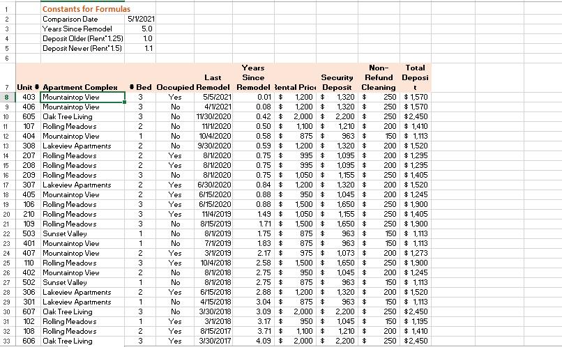
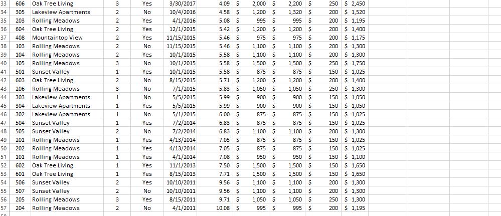
2	Before subtotalling the data, you need to sort the data. Select the Summary sheet. Sort the data by Apartment Complex in alphabetical order and further sort it by # Bed (the number of bedrooms) from smallest to largest.
3	You want to use the Subtotal feature to display the average total deposit by number of bedrooms for each apartment complex. Use the Subtotal feature to insert subtotal rows by Apartment Complex to calculate the average Total Deposit. Add a second subtotal (without removing the first subtotal) by # Bed to calculate the average Total Deposit by the number of bedrooms.
4	Use the outline symbols to display only the subtotal rows. Create an automatic outline and collapse the outline above Total Deposit.
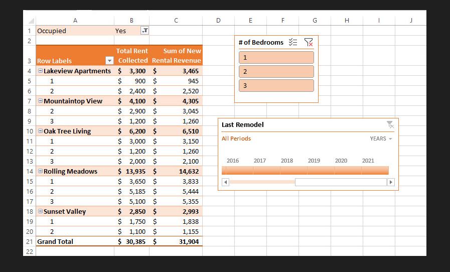
5	You want to create a PivotTable to determine the total monthly rental revenue for occupied apartments. Display the Rentals sheet and create a blank PivotTable on a new worksheet to the left of the Rentals sheet. Change the name of the worksheet to Rental Revenue. Name the PivotTable Rental Revenue.
6	Display the Apartment Complex and # Bed fields in Rows and the Rental Price field as Values.
7	Format the Sum of Rental Price for Accounting Number Format with zero decimal places and enter the custom name Total Rent Collected.
8	Select the Occupied field for the filter and set the filter to Yes to display data for occupied apartments.
9	You want to calculate the total monthly rental revenue if the rates increase by 5% for the occupied apartments. Insert a calculated field to multiply the Rental Price by 1.05. Change the name to New Rental Revenue. Apply Accounting Number Format with zero decimal places.
10	Select the range B3:C3 and apply these formats: wrap text, Align Right horizontal alignment, and 30 row height. Select column B and set 9.29 column width. Select column C and set 14.43 column width.
11	Apply Light Orange, Pivot Style Medium 10 to the PivotTable and display banded rows.
12	Insert a slicer for # Bed so that you can filter the dataset by number of bedrooms. Change the slicer caption to # of Bedrooms.
13	Change the slicer height to 1.4 inches and width to 1.75 inches. Apply Light Orange, Slicer Style Light 2. Cut the slicer and paste it in cell E2.
14	Insert a timeline for the Last Remodel field. Change the time period to YEARS. Apply Light Orange, Timeline Style Light 2. Change the timeline height to 1.4 inches and with to 3.75 inches.
15	The Databases sheet contains two tables. You will create a relationship between those tables. Display the Databases sheet. Create a relationship between the APARTMENTS table using the Code field and the COMPLEX table using the Code field.
16	You want to create a PivotTable from the related tables. Create a PivotTable using the data model on a new sheet. Change the sheet name to Bedrooms. Name the PivotTable BedroomData.
17	Select the Apartment Name field from the COMPLEX table for Rows, the # Bed field for Columns, and the # Bed field as Values. This will display the number of apartments with the specified number of bedrooms per apartment complex. Display the values as a percentage of row totals.
18	Create a Clustered Column PivotChart. Cut the chart and paste it in cell A13.
19	Select the 3-bedroom data series and apply the Black, Text 1, Lighter 50% solid fill color. Apply Black, Text 1 font color to the vertical axis and category axis. Change the chart height to 3 inches and the width to 5 inches, if necessary. Hide the field buttons in the PivotChart.
20	Create a footer on all worksheets with your name in the left, the sheet name code in the center, and the file name code in the right.
21	Save and close Exp19_Excel_Ch05_Cap_Apartments.xlsx. Exit Excel. Submit the file as directed.

    

-23+56 1 4 ~=~222222=22*222*88588 7 Unit Apartment Complex 403 Mountaintop View 406 Mountaintop View 605 Oak Tree Living 107 Rolling Meadows 404 Mountaintop View 308 Lakeview Apartments 207 Rolling Meadows 208 Rolling Meadows 209 Rolling Meadows 307 Lakeview Apartments 405 Mountaintop View Rolling Meadows Rolling Meadows 106 210 109 Rolling Meadows 503 Sunset Valley 23 401 Mountaintop View 24 407 Mountaintop View Rolling Meadows Mountaintop View 110 502 Sunset Valley 306 301 607 9 10 11 12 13 14 15 16 17 18 19 20 21 26 402 27 29 30 31 32 33 Constants for Formulas Comparison Date 102 108 606 Years Since Remodel Deposit Older (Rent 1.25) Deposit Newer (Rent 1.5) Lakeview Apartments Lakeview Apartments Oak Tree Living Rolling Meadows Rolling Meadows Oak Tree Living 5/1/2021 5.0 1.0 1.1 Last * Bed Occupied Remodel Yes 3 3 No No 5/5/2021 4/1/2021 11/30/2020 11/1/2020 10/4/2020 9/30/2020 No No No 8/1/2020 Yes Yes No 8/1/2020 8/1/2020 MMMN-NNN 3 2 1 2 2 2 MNA 3 2 2 3 3 MOTT 3 1 1 2 NWN 3 2 -N 1 2 1 3 1 N3 2 Yes Yes Yes Yes No No No Yes Yes No No Yes No No Yes Yes Yes 6/30/2020 6/15/2020 6/15/2020 11/4/2019 8/15/2019 8/1/2019 7/1/2019 3/1/2019 10/4/2018 8/1/2018 8/1/2018 6/15/2018 4/15/2018 3/30/2018 3/1/2018 8/15/2017 3/30/2017 Years Since Security Remodel lental Price Deposit 0.01 $ 1,200 $ 1,320 $ 0.08 $ 0.42 $ 0.50 $ 0.58 $ 0.59 $ 0.75 $ 0.75 $ 0.75 $ 0.84 $ 0.88 $ 0.88 $ 1.49 $ 1.71 $ 1.75 $ 1.83 $ 2.17 $ 2.58 $ 2.75 $ 2.75 $ 2.88 $ 3.04 $ 3.09 $ Non- Total Refund Deposi Cleaning 3.17 $ 3.71 $ 4.09 $ 1,320 $ 1,200 $ 2,000 $ 2,200 $ 1,100 $ 1,210 $ 875 $ 963 $ 1,200 $ 1,320 $ 995 $ 1,095 $ 995 $ 1,050 $ 1,200 $ 1,095 $ 1,155 $ 1,320 $ 1,045 $ 1,650 $ 1,155 $ 950 $ 1,500 $ 1,050 $ 1,500 $ 1,650 $ 875 $ 963 $ 875 $ 963 $ 975 $ 1,073 $ 1,500 $ 950 $ 875 $ 1,200 $ 875 $ 2,000 $ 950 $ 1,100 $ 2,000 $ 1,650 $ 1,045 $ 963 $ 1,320 $ 963 $ 2,200 $ 1,045 $ 1,210 $ 2,200 $ t 250 $1,570 250 $ 1,570 250 $2,450 200 $ 1,410 150 1,113 200 $1,520 200 $1,295 200 $1,295 250 $1,405 200 $1,520 200 $1,245 250 $1,900 250 $1,405 250 $1,900 150 $ 1,113 150 $ 1,113 200 $1,273 250 $1,900 200 $1,245 150 $ 1,113 200 $1,520 150 $ 1,113 250 $2,450 150 $ 1,195 200 $ 1,410 250 $2,450