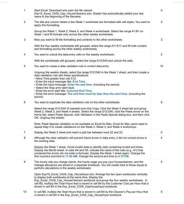
Question: Start Excel. Download and open the file named Exp19_Excel_Ch09_Cap_HouseCleaners.xfsx. Grader has automatically added your last name to the beginning of the filename. 1 2


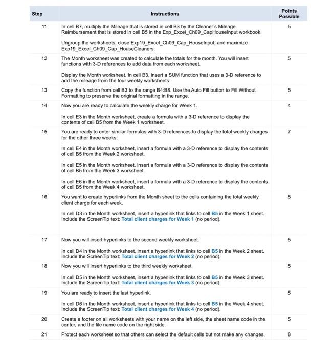
Start Excel. Download and open the file named Exp19_Excel_Ch09_Cap_HouseCleaners.xfsx. Grader has automatically added your last name to the beginning of the filename. 1 2 The title and column labels in the Week 1 worksheet are formatted with cell styles. You want to apply this formatting. Group the Week 1, Week 2, Week 3, and Week 4 worksheets. Select the range A1:B1 on Week 1 and fill formats only across the other weekly worksheets. 3 Now you want to fill the formatting and contents to the other worksheets. 3 With the four weekly worksheets still grouped, select the range A11:E11 and fill both content and formatting across the other weekly worksheets. 4 You want to unlock the data-entry cells on the weekly worksheets. 2 With the worksheets still grouped, select the range A12:D40 and unlock the cells. 5 You want to create a data validation rule to control data entry. 10 Ungroup the weekly sheets, select the range D12:D40 in the Week 1 sheet, and then create a data validation rule with these specifications: Allow Time greater than cell C12. Enter the input message title: End Time. Enter the input message: Enter the end time. (including the period). Select the Stop error alert style. Enter the error alert title: Incorrect End Time. Enter the error message: The end time must be later than the start time. (including the period). You want to duplicate the data validation rule on the other worksheets. Select the range D12:D40 (if needed) and click Copy. Click the Week 2 sheet tab and group Week 2, Week 3, and Week 4 sheets. Select the range D12:D40, click the Paste arrow on the Home tab, select Paste Special, click Validation in the Paste Special dialog box, and then click OK. Ungroup the sheets. Note: Paste Special validation is not available on Excel for Mac. Excel for Mac users need to repeat Step 5 to create validations on the Week 2, Week 3, and Week 4 workshops. 7 Display the Week 2 sheet and insert a split bar between rows 22 and 23. 8 Although the data validation will prevent future errors in data entry, it did not correct errors in the existing data. Display the Week 1 sheet. Circle invalid data to identify cells containing invalid end times. Display the Month sheet. In cells H4 and H5, indicate the name of the cells (e.g., A1) that contained the errors (do not enter a formula). Display the Week 1 sheet again. Change the first incorrect end time to 11:00 AM. Change the second end time to 4:15 PM. 9 The hourly rate you charge clients, the hourly wage you pay your housecleaners, and the mileage allowance are stored in a separate workbook. You will create links to those inputs to perform calculations in the weekly worksheets. Open Exp19_Excel_Ch09_Cap_Houselnput.xlsx. Arrange the two open workbooks vertically to display both workbooks at the same time. Display the Exp_Excel_Ch09_Cap_HouseCleaners workbook and group the four weekly worksheets. In cell B5, multiply the Total Hours that is stored in cell B4 by the Customer Cost per Hour that is stored in cell B3 in the Exp_Excel_Ch09_CapHouselnput workbook. In cell B6, multiply the Total Hours that is stored in cell B4 by the Cleaner's Pay per Hour that is stored in cell B4 in the Exp_Excel_Ch09_Cap_Houselnput workbook. 10 Points Step Instructions Possible In cell B7, multiply the Mileage that is stored in cell B3 by the Cleaner's Mileage Reimbursement that is stored in cell B5 in the Exp_Excel_Ch09 CapHouselnput workbook. 11 Ungroup the worksheets, close Exp19_Excel_Ch09_Cap_Houselnput, and maximize Exp19_Excel_Ch09_Cap HouseCleaners. 12 The Month worksheet was created to calculate the totals for the month. You will insert functions with 3-D references to add data from each worksheet. Display the Month worksheet. In cell B3, insert a SUM function that uses a 3-D reference to add the mileage from the four weekly worksheets. 13 Copy the function from cell B3 to the range B4:B8. Use the Auto Fill button to Fill Without Formatting to preserve the original formatting in the range. 14 Now you are ready to calculate the weekly charge for Week 1. In cell E3 in the Month worksheet, create a formula with a 3-D reference to display the contents of cell B5 from the Week 1 worksheet. 15 You are ready to enter similar formulas with 3-D references to display the total weekly charges for the other three weeks. 7 In cell E4 in the Month worksheet, insert a formula with a 3-D reference to display the contents of cell B5 from the Week 2 worksheet. In cell E5 in the Month worksheet, insert a formula with a 3-D reference to display the contents of cell B5 from the Week 3 worksheet. In cell E6 in the Month worksheet, insert a formula with a 3-D reference to display the contents of cell B5 from the Week 4 worksheet. 16 You want to create hyperlinks from the Month sheet to the cells containing the total weekly client charge for each week. In cell D3 in the Month worksheet, insert a hyperlink that links to cell B5 in the Week 1 sheet. Include the ScreenTip text: Total client charges for Week 1 (no period). 17 Now you will insert hyperlinks to the second weekly worksheet. 5 In cell D4 in the Month worksheet, insert a hyperlink that links to cell B5 in the Week 2 sheet. Include the Screen Tip text: Total client charges for Week 2 (no period). 18 Now you will insert hyperlinks to the third weekly worksheet. In cell D5 in the Month worksheet, insert a hyperlink that links to cell B5 in the Week 3 sheet. Include the ScreenTip text: Total client charges for Week 3 (no period). 19 You are ready to insert the last hyperlink. In cell D6 in the Month worksheet, insert a hyperlink that links to cell B5 in the Week 4 sheet. Include the ScreenTip text: Total client charges for Week 4 (no period). 20 Create a footer on all worksheets with your name on the left side, the sheet name code in the center, and the file name code on the right side. 21 Protect each worksheet so that others can select the default cells but not make any changes. 8.
Step by Step Solution
3.37 Rating (156 Votes )
There are 3 Steps involved in it

Get step-by-step solutions from verified subject matter experts


