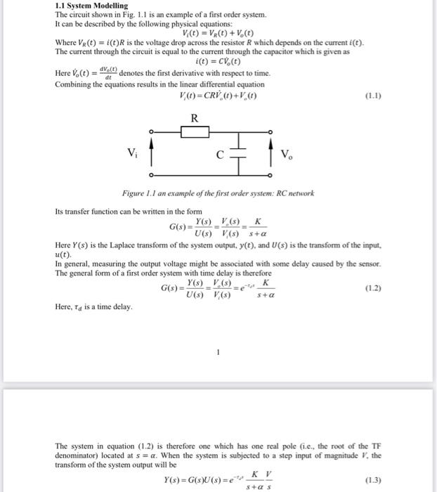
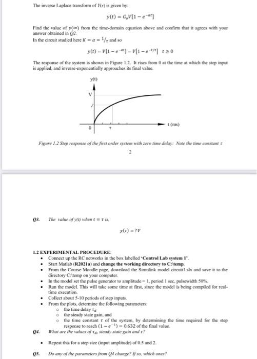
1.1 System Modelling The circuit shown in Fig. 1.1 is an example of a first order system. It can be described by the following physical equations: V(t) = Vr(t) + V (1) Where Vr(t) = i(t) is the voltage drop across the resistor R which depends on the current i(t). RS The current through the circuit is equal to the current through the capacitor which is given as i(t) = CV.C.) denotes the first derivative with respect to time. Combining the equations results in the linear differential equation VC)=CR (1)+V,0 (1.1) Here Vo(t) = V...) R V V. '! Figure 1.1 an example of the first order system: RC network Its transfer function can be written in the form G(s) Y(s)_V,(s) * U(s) V(s) sta Here Y() is the Laplace transform of the system output, y(t), and U(5) is the transform of the input, u(t). In general, measuring the output voltage might be associated with some delay caused by the sensor. The general form of a first order system with time delay is therefore Y(s) V (8) K (1.2) sta Here, Ta is a time delay. G(s) - U(8) V(8) 1 The system in equation (1.2) is therefore one which has one real pole (i.c., the root of the TF denominator) located at s = a. When the system is subjected to a step input of magnitude V. the transform of the system output will be KV Y(s)=G($)U(s) = (1.3) sas The inverse Laplace transform of Ps) is given by: y(t) = G,V[1 - Find the value of y() from the time-domain equation above and confirm that it agree with your answer obtained in 02 In the circuit studied here X = 2 = 1 and so y(t) = V1 -2-) = V1 -2- +20 The response of the system is shown in Figure 1.2 lt rises from at the time which the step input is applied, and inverse-exponentially approaches its final value C (ms) 0 5 Figure 1.2 Step response of the first order system with zero time delay: Note the time constant 03. The value of when trix VT) =? 1.2 EXPERIMENTAL PROCEDURE: Connect up the RC networks in the box labelled Control Lab system !". Start Matlab (R2021a) and change the working directory to C:temp. From the Course Moodle pagc, download the Simulink model circuitiske and save it to the directory C temp on your computer In the model set the pulse generator to amplitude - 1. period 1 sec. pulsewidth 50% Run the model. This will take some time at first, since the model is being compiled for real- time execution Collect about 5-10 periods of step inputs. From the plots, determine the following parameters o the time delay To the steady state gain, and the time constant of the system, by determining the time required for the step response to reach (1 - -) - 0.632 of the final value. 04. What are the values of Tg steady stale gain and t Repeat this for a step size (input amplitude) of 0.5 and 2 Os. Do any of the parameters from change? If so, which ones