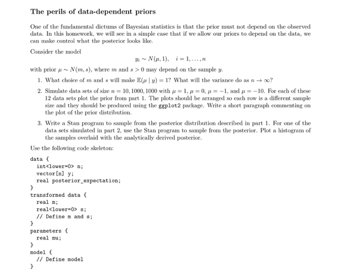
The perils of data-dependent priors One of the fundamental dictums of Bayesian statistics is that the prior must not depend on the observed data. In this homework, we will see in a simple case that if we allow our priors to depend on the data, we can make control what the posterior looks like. Consider the model Yi - N(u, 1), i= 1,...,n with prior u- N(m, s), where m and s >0 may depend on the sample y. 1. What choice of m and s will make E(u | 3) = 1? What will the variance do as n oo? 2. Simulate data sets of size n = 10, 1000, 1000 with u = 1, j = 0, = -1, and u = -10. For each of these 12 data sets plot the prior from part 1. The plots should be arranged so each row is a different sample size and they should be produced using the ggplot2 package. Write a short paragraph commenting on the plot of the prior distribution. 3. Write a Stan program to sample from the posterior distribution described in part 1. For one of the data sets simulated in part 2, use the Stan program to sample from the posterior. Plot a histogram of the samples overlaid with the analytically derived posterior. Use the following code skeleton: data { int n; vector [n] y; real posterior_expectation; transformed data { real m; real s; // Define m and s; parameters { real mu; model { // Define model The perils of data-dependent priors One of the fundamental dictums of Bayesian statistics is that the prior must not depend on the observed data. In this homework, we will see in a simple case that if we allow our priors to depend on the data, we can make control what the posterior looks like. Consider the model Yi - N(u, 1), i= 1,...,n with prior u- N(m, s), where m and s >0 may depend on the sample y. 1. What choice of m and s will make E(u | 3) = 1? What will the variance do as n oo? 2. Simulate data sets of size n = 10, 1000, 1000 with u = 1, j = 0, = -1, and u = -10. For each of these 12 data sets plot the prior from part 1. The plots should be arranged so each row is a different sample size and they should be produced using the ggplot2 package. Write a short paragraph commenting on the plot of the prior distribution. 3. Write a Stan program to sample from the posterior distribution described in part 1. For one of the data sets simulated in part 2, use the Stan program to sample from the posterior. Plot a histogram of the samples overlaid with the analytically derived posterior. Use the following code skeleton: data { int n; vector [n] y; real posterior_expectation; transformed data { real m; real s; // Define m and s; parameters { real mu; model { // Define model