New Semester Started Get 50% OFF Study Help! --h --m --s Claim Now

Question Answers

Textbooks

Find textbooks, questions and answers

Oops, something went wrong!

Change your search query and then try again

Result Not Found

Books FREE
Study Help
Tutors
AI Study Planner NEW
Sell Books

Search
Sign In
Register

study help
statistics
statistical analysis

Statistical Analysis Of Financial Data 1st Edition James Gentle - Solutions

Obtain the Consumer Price Index for All Urban Consumers: All Items for the period January 1, 2000 to December 31, 2018. These monthly data, reported as of the first of the month, are available as CPIAUCSL from FRED. Compute the simple monthly returns for this period.Now obtain the 15-Year Fixed
Work out the autocovariance \(\gamma(h)\) for the MA(2) model.
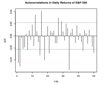
Obtain the S\&P 500 Index daily closes for the period from January 1987 to December 2017 and compute the log returns. These are the data shown in Figure 1.30. Fit an MA(2) model to the returns. Comment on the fit and this method of analysis generally. Can ARMA models add meaningful insight into
(a) In the AR(1) model \(x_{t}=\phi_{0}+\phi_{1} x_{t-1}+w_{t}\), with \(\phi_{1}
(a) For each pair of coefficients, write the characteristic polynomial, evaluate the discriminant, determine the characteristic roots, and compute their moduli.i. \(\phi_{1}=\sqrt{2} ; \phi_{2}=-1 / 2\)ii. \(\phi_{1}=9 / 8 ; \phi_{2}=-1 / 4\)iii. \(\phi_{1}=1 / 4 ; \phi_{2}=1 / 2\)iv. \(\phi_{1}=-1
For each pair of coefficients, determine the ACF up to the lag specified and comment on the results. You may want to use the R function ARMAacf.(a) \(\phi_{1}=\sqrt{2} ; \phi_{2}=-1 / 2\); to lag 15(b) \(\phi_{1}=9 / 8 ; \phi_{2}=-1 / 4\); to lag 15(c) \(\phi_{1}=1 / 4 ; \phi_{2}=1 / 2\); to lag
(a) For an \(\mathrm{AR}(2)\) model, show that \(\phi(3,3)=0\) in equation (5.129).(b) For an \(\mathrm{AR}(2)\) model with \(\phi_{1}=\sqrt{2} ; \phi_{2}=-1 / 2\), compute the PACF. You may want to use the \(\mathrm{R}\) function
(a) Show that the denominator in the solutions to the Yule-Walker equations (5.119) and (5.120), \((\gamma(0))^{2}-(\gamma(1))^{2}\), is positive and less than 1.(b) Suppose that for a certain process, we have \(\gamma(0)=2, \gamma(1)=\) 0.5 , and \(\gamma(2)=0.9\).If the process is an
Some previous exercises have involved model (theoretical) properties of an \(\mathrm{AR}(2)\) process. In this exercise, you are to use simulated data from an \(\mathrm{AR}(2)\) process. For each part of this exercise, generate 1,000 observations from the causal AR(2) model\[ x_{t}=\sqrt{2}
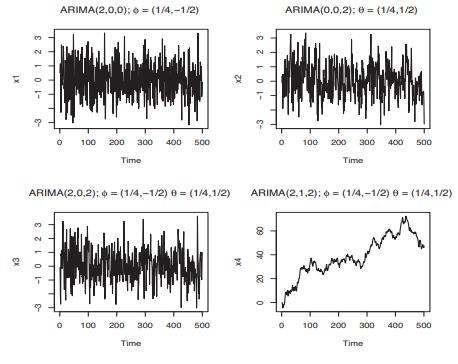
As seen from Figure 5.13, there may be very little visual difference in ARMA models with different values of the coefficients. ARIMA models with \(d>0\) are generally nonstationary, however.(a) Generate 500 values of an \(\operatorname{ARIMA}(2,1,2)\) process with Gaussian innovations and
(a) Generate four sets of ARIMA data using the same models as used to produce the series shown in Figure 5.13, except for the innovations, use a t distribution with 5 degrees of freedom.Plot the four series in a manner similar to Figure 5.13, in which a normal distribution was used.Comment on the
The weekly yields of Moody's seasoned Aaa corporate bonds, the yields of 3-month Treasury bills, the yields of 2 -year Treasury notes, the yields of 10 -year Treasury notes, and the yields of 30-year Treasury bonds for the years 2008 through 2018.Using OLS, fit the linear regression of the change
Consider the regression of the US gross domestic product (GDP) on some other economic measures relating to the labor force.There are various measure of the GDP. We will use the dataset GDP at FRED, which is a quarterly, seasonally-adjusted series begun in 1947 and maintained by the US Bureau of
Obtain the weekly log returns of the S\&P 500 index for the period January 1, 1978 through December 31, 2017, and compute the weekly \(\log\) returns. (a) Test for an ARCH effect in this time series.(b) Fit an ARIMA \((1,1,1)+\operatorname{GARCH}(1,1)\) model to the weekly log returns of the S\&P
(a) i. Generate a random walk of length 10 and perform an augmented Dickey-Fuller test on the series for a unit root.ii. Generate a random walk of length 100 and perform an augmented Dickey-Fuller test on the series for a unit root.iii. Generate a random walk of length 1,000 and perform an
(a) Obtain the daily adjusted closing prices of MSFT for the period January 1, 2007, through December 31, 2007.i. Perform an augmented Dickey-Fuller test on the series of adjusted closing prices for a unit root.ii. Now compute the returns for that period and perform an augmented Dickey-Fuller test
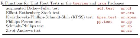
Obtain the quarterly, seasonally-adjusted US gross domestic product (GDP) in the FRED dataset GDP (beginning in 1947). Test for a unit root in the \(\log \mathrm{CDF}\).Use six different tests: augmented Dickey-Fuller, Elliott-Rothenberg-Stock, Kwiatkowski-Phillips-Schmidt-Shin (KPSS),
Simulate a random walk \(\left\{z_{t}\right\}\) of length 500 . Now generate two series, \(\left\{x_{t}\right\}\) and \(\left\{y_{t}\right\}\), each of which follows the random walk with an additive white noise, one with variance \(\sigma_{1}^{2}=1\) and the other with variance
Obtain the exchange rates for the US dollar versus the euro from 1999-01-04 to the present and the exchange rates for the Japanese yen versus the US dollar for the same period, and test for cointegration.What are your conclusions? Discuss.
Consider the simple discrete distribution of the random variable \(X\) with probability function as given in equation (3.18). Make two transformations,\[ Y=2 X+1 \]and\[ Z=X^{2}+1 \](a) Using the respective probability functions, compute \(\mathrm{E}(X)\), \(\mathrm{V}(X), \mathrm{E}(Y),
Let \(X\) be a random variable and let \(\mathrm{E}(X)=\theta eq 0\) and \(\mathrm{V}(X)=\) \(\tau^{2}>0\).Let \(b\) be a constant such that \(0
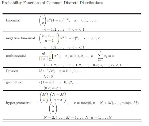
(a) Show that the variance of the Poisson distribution whose probability function is shown in Table 3.1 is \(\lambda\), the same as the mean of the distribution.(b) Show that the mean of the \(\mathrm{U}(0,1)\) distribution is \(1 / 2\) and the variance is \(1 / 12\).(c) Show that the mean and
(a) Determine the survival function and the hazard function for the Weibull distribution with parameters \(\alpha\) and \(\beta\).(b) Determine the hazard function for the exponential distribution with parameter \(\lambda\).What are the implications of this; that is, in what kinds of situations
(a) Let \(X\) have the triangular distribution (see Exercise 3.3e.) Let \(Y=2 X+3\). Determine the PDF of \(Y\), show that your function is a \(\mathrm{PDF}\), and compute \(\mathrm{E}(Y)\) and \(\mathrm{V}(Y)\).(b) Let \(X\) have the triangular distribution.Let \(Z=X^{2}\). Determine the PDF of
Suppose the price of stock XYZ is \(\$ 100\), suppose that the standard deviation of the daily returns of XYZ is 0.002 , and suppose that the risk-free interest rate \(r_{\mathrm{F}}\) is \(1 \%\).(a) What is the (annualized) volatility \(\sigma\) of XYZ?(b) Assume a unit of time as one year and a
(a) Plot on the same set of axes, using different line types and/or different colors, the PDFs of a standard normal distribution, a \(t\) with 10 degrees of freedom, a \(t\) with 2 degrees of freedom, and a Cauchy.Briefly discuss the plots.(b) Show that the mean and variance of the Cauchy
(a) Consider a normal distribution with mean 100 and variance 100. Write out the CDF of the threshold exceedance distribution with respect to 120 (two standard deviations above the mean). Just use symbols for functions that cannot be evaluated in closed form.(b) Use R or another computer program to
(a) For the standard normal distribution, plot the PDF in equation (3.101) for four values of \(\alpha, \alpha=-1, \frac{1}{2}, 1,2\), along with the PDF of the standard normal.(b) Generate 1,000 realizations of the maximum of two standard normal random variables. (For each, you could use \(\max
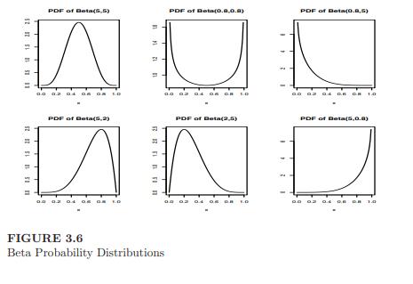
(a) Generate 10,000 random variables following the beta \((5,5)\), the beta \((0.8,0.8)\), the beta \((0.8,5)\), the beta \((5,2)\), the beta \((2,5)\), and the beta( \(5,0.8)\) distributions.Fit kernel densities to each one, and produce six plots of the empirical densities, similar to the
Consider a random sample of size \(n\) from the unit Pareto distribution with PDF\[ f(x)=2 x^{-2} \quad \text { for } 0 \leq x \]that is, for the Pareto with \(\alpha=2\) and \(\gamma=1\).(a) Write the cumulative distribution function for the maximum order statistic \(X_{(n: n)}\) in the sample.(b)
(a) Show formally that the median of a lognormal distribution with parameters \(\mu\) and \(\sigma\) is \(\mathrm{e}^{\mu}\).Now generate 1,000 numbers that simulate a lognormal distribution with parameters 3 and 2. (Note that these parameters, while they are often denoted as \(\mu\) and
(a) Let \(X\) be a random variable with a location-scale t distribution with 3 degrees of freedom, location 100, and scale 10.i. What is the probability that \(X\) is less than or equal to 110 ? ii. What is the 0.25 quantile of \(X\) ?(b) Generate a sample of 1,000 random numbers following the
(a) Write a function to generate multivariate normal random numbers of a specified dimension and with a specified covariance matrix. The first statement for an \(\mathrm{R}\) function should be rmulvnorm The R function chol computes the transformation matrix from Sigma. (The function rmulvnorm has
Suppose \(X\) has a bivariate normal distribution, with mean 0 , \(\mathrm{V}\left(X_{1}\right)=\sigma_{1}^{2}\), and \(\mathrm{V}\left(X_{2}\right)=\sigma_{2}^{2}\). Let \(F_{1}\) and \(F_{2}\) be the CDFs of two continuous univariate distributions.Now, let\[ Y=\left(Y_{1},
Let \(m=2^{31}-1, j=5\), and \(k=17\). Let\[ \left\{x_{1}, x_{2}, \ldots, x_{17}\right\}=\{m / 17-1,2 m / 17-1, \ldots, m-1\} \]Now for \(i=18,19, \ldots, 1017\). Compute a "random sample" of size 1,000 in this manner.\(x[i]
(a) Generate 1,000 random numbers from the triangular distribution. (The PDF is given in equation (3.28).) Produce a histogram and compute some summary statistics.\(f_X(x)= \begin{cases}1-|x| & \text { for }-1
Use a Sobol' sequence to generate 1,000 quasirandom numbers from the triangular distribution, as in Exercise 3.17a. (A Sobol' generator is in the \(\mathrm{R}\) package randtoolbox.)Produce a histogram and compute some summary statistics. Can you tell any differences in the pseudorandom numbers of
Suppose the price of stock XYZ is \(\$ 100\). Suppose that the daily \(\log\) returns follow a location-scale t distribution with mean 0 , scale 0.002, and degrees of freedom 6 . Assume that the daily log returns are sequentially independent. (A large assumption!)(a) Generate a random sequence of
Consider the daily prices of XYZ, as in Exercise 3.19, and assume the same location-scale \(t\) distribution for the returns.Generate 1,000 random sequences of 253 daily prices of XYZ, each starting at \(\$ 100\).Before answering any of the following questions, read all questions so as to
Suppose that the daily log returns of an asset follow a location-scale \(\mathrm{t}\) distribution with mean 0 , scale 0.002 , and degrees of freedom 6, and assume that the daily log returns are sequentially independent. Suppose further that the prices of the asset are subject to random shocks that
We form a portfolio consisting of two stocks, XYZ, and \(\mathrm{ABC}\) whose daily log returns of the stock \(\mathrm{ABC}\) have a location-scale \(t\) distribution with mean 0 , scale 0.005 , and degrees of freedom 3 .Assume that the returns are sequentially independent, and suppose further that
During the course of a year, the yields of US Treasuries vary. Which do you expect to vary most: Bills, Notes, or Bonds?Why do you answer as you do?
Suppose a coupon bond with a par value of \(\$ 1,000\) pays a semiannual coupon payment of \(\$ 20\). (This is fair-priced at issue at an annual rate of \(4 \%\).)(a) Now, suppose the annual interest rate has risen to 6\% (3\% semiannually). What is the fair market price of this bond if the
Suppose the price of one share of XYZ was \(\$ 100\) on January 1 and was \(\$ 110\) on July 1. Suppose further that at the end of that year, the simple return for the stock was \(5 \%\).(a) As of July 1, what was the simple one-period return?(b) As of July 1, what was the annualized simple
Assume that an asset has a simple return in one period of \(R_{1}\), and in a subsequent period of equal length has a simple return of \(R_{2}\). What is the total return of the asset over the two periods? (Compare equation (1.26) for \(\log\) returns.)\(r=\sum_{i=2}^n r_i . \tag{1.26}\)
Assume a portfolio of two assets with weights \(w_{1}\) and \(w_{2}\), and having \(\log\) returns of \(r_{1}\) and \(r_{2}\). Show, by an example if you wish, that the \(\log\) return of the portfolio is not necessarily \(w_{1} r_{1}+w_{2} r_{2}\) as in the case of simple single-period returns in
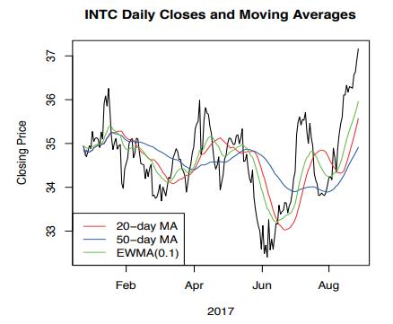
Suppose the stock XYZ has been generally increasing in price over the past few months. In a time series graph of the stock price, its 20 -day moving average, and its 50-day moving average, as in Figure 1.9, which curve will be highest, the price, the 20-day moving average, or the 50-day moving
Suppose a common share of XYZ closed at \(\$ 40.00\) on December 31, and on April 1 of the following year, the stock split two-for-one. The stock closed at \(\$ 21.00\) on December 31 of that following year.(a) Suppose the company did not pay any dividends, returned no capital, and no other splits
On January 3, 2017, the closing price of Goldman Sachs (GS) was 241.57 and the closing value of the DJIA was 19,881.76. The DJIA divisor at that time was 0.14523396877348 .(a) Suppose that GS split two-for-one at the close on that day (and no other components of the DJIA split). What would be the
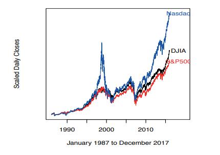
Explain the similarities and the divergences in the three indexes shown in Figure 1.10.Figure 1.10: Scaled Daily Closes A 1990 2000 2010 January 1987 to December 2017 Nasdad DJIA G&P500
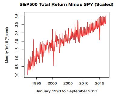
In Figure 1.14, we compared the daily rates of return on the adjusted closing prices of SPY with the daily rates of return on the S&P 500 Total Return. Why is that appropriate (instead of, for example, using the rates of return on the S\&P 500 Index)?Figure 1.14: Monthly Deficit (Percent)
The risk of a portfolio consisting of two risky assets with risks \(\sigma_{1}\) and \(\sigma_{2}\) and correlation \(ho\) in proportions \(w_{1}\) and \(w_{2}\) is\[ \sigma_{\mathrm{P}}=\sqrt{w_{1}^{2} \sigma_{1}^{2}+w_{2}^{2} \sigma_{2}^{2}+2 w_{1} w_{2} ho \sigma_{1} \sigma_{2}} \]Let us
Explain why each position in the following pairs of positions is a hedge against the other.(a) long 200 shares of MSFT and long 1 MSFT put (at any strike price and at any future expiry)(b) short 200 shares of MSFT and short 2 MSFT puts (at any strike price and at any future expiry) (This is not a
Suppose that on 2017-04-04 the closing price of MSFT was 65.00.On that day, the price of the October 70 call was 1.65.On that day, the price of the October 60 put was 2.21.In 2017, the date of expiration of October stock options was October 20.In each hypothetical case below, state whether the
(a) Suppose that stock XYZ is trading at \(\$ 80.00\) on February 12 , and its price increases to \(\$ 83.00\) on February 14. This \(\$ 3.00\) increase will affect the price of options on the stock. Consider six different call options on the stock: the February 80 call, the February 95 call, the
Several widely-cited empirical studies have shown that approximately \(75 \%\) to \(80 \%\) of stock options held until expiration expire worthless (out of the money). Based on these studies, many have concluded that long option positions are on the whole unprofitable. Give two counter-arguments
Suppose a company has 10 employees who make \(\$ 10\) an hour, a manager who makes \(\$ 100\) an hour, and a director who makes \(\$ 280\) an hour.(a) What is the mean wage?(b) What are the \(5 \%\) trimmed and Winsorized means?(c) What are the \(15 \%\) trimmed and Winsorized means?
Explain why quantile-based measures such as the IQR and Bowley's skewness coefficient are less affected by heavy-tailed distributions than are moment-based measures such as the standard deviation or the ordinary measure of skewness (Pearson's).
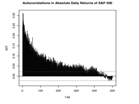
Explain how absolute returns can have large autocorrelations, as shown in Figure 1.31, when the returns themselves are uncorrelated. Does this make sense?FIGURE 1.31: ACF ON 0.00 0.05 0.15 0.10 0.25 0.20 0.30 Autocorrelations in Absolute Daily Returns of S&P 500 0 100 200 300 400 500 Lag
Does the VIX seem to exhibit a mean reversion? When the VIX is 12 or less, does it appear to be more likely that it will be larger (than 12) within the next 6 months than when it is 25 or greater to be larger (than 25 )?
Obtain closing data for NFLX for the first calendar quarter 2018 (January 2 through March 30). Compute the simple returns and the \(\log\) returns (unadjusted).Compute the mean, median, standard deviation, skewness, and kurtosis for both types of returns.Based on those statistics, what can you say
(a) For a few different values of the standard deviation in normal distributions, compute the MAD. What is the ratio of the standard deviation to MAD? (Perform these computations for the theoretical normal distribution; not for samples.)Comment on your findings.(b) For a few different values of the
Obtain the SPY, UPRO, and SDS daily closing prices (unadjusted) for the periods from their inception through 2018. SPY tracks the S\&P 500; UPRO daily returns track three times the S\&P 500 daily returns; and SDS daily returns track twice the negative of the S\&P 500 one day returns. (SPY is a SPDR
Plot the ECDF of the daily simple returns for NFLX for the first calendar quarter 2018. Superimpose on the same plot a plot of the normal CDF with mean the same as the sample mean of the NFLX daily simple returns and standard deviation the same as the standard deviation of the NFLX daily simple
Consider the small set of numbers\[ 11,14,16,17,18,19,21,24 \](a) Compute the 0.25 quantile of this sample using all nine different interpretations of equation (2.11) that are provided in the \(R\) function quantile. (Use the type argument.)(b) What are the first and third quartiles using the
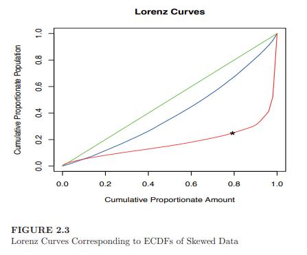
We emphasized the importance of recognizing whether time is a fundamental component of data, and we suggested a simple plot, illustrated in Figure 2.3 to use to decide how important time may be.Generally, we know that price data on a stock are highly dependent on time, but the returns on a stock
Obtain the INTC, MSFT, and ^IXIC adjusted closing prices for the period 1988 through 2017.Plot these prices as time series data on the same set of axes. Use different colors or line types for the different series, and print a legend on your graph.
Produce three or four histograms of the daily returns for NFLX for the first calendar quarter 2018, using different bin widths of your choice.Which bin width seems best?
Using the bin width you selected in Exercise 2.8 (or just any old bin width; it is not important for the purpose of this exercise), produce two histograms of the daily \(\log\) returns for NFLX for the full year 2018. For one, make a frequency histogram and for the other, a density histogram.What
Using the daily returns for NFLX for the first calendar quarter 2018, fit a kernel density using four different smoothing parameter values and two different kernels. (Choose the values and the kernels "intelligently".)Comment on the differences.Describe the distribution of the NFLX returns.
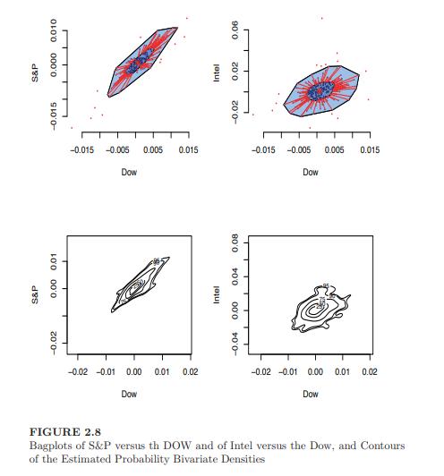
Obtain closing data and compute daily returns for NFLX and for GLD for the first calendar quarter 2018.(a) Bivariate boxplot; bagplot.Produce a bagplot of the returns of NFLX and GLD for that period.(b) Bivariate kernel density estimators.Choose four different smoothing matrices for a bivariate
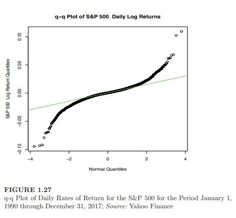
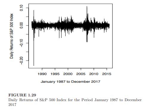
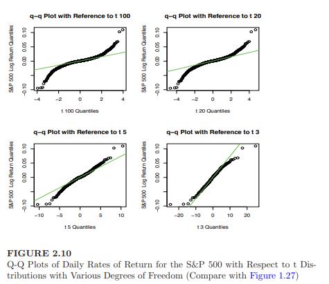
Obtain the daily closes of the S\&P 500 from January 1, 1990, through December 31, 2017, and compute the daily log returns. These are the data used in Figure 1.27 on page 92 and a subset of those shown in Figure 1.29 on page 99. Q-q plots of the data are shown in Figure 1.27 and Figure 2.10.(a)
Obtain closing data and compute daily returns for the full year 2017 for the S\&P 500 and for First Solar (FSLR), which was a component of the index during that period. FSLR has historically been one of the most volatile stocks in the index.(a) Produce a q-q plot with respect to a normal
Obtain the daily closes of the Nasdaq Composite ( \({ }^{\text {IXIC) for the }}\) period 1988 through 2017. Compute the daily log returns.(a) Compute the mean, standard deviation, skewness, and kurtosis of the returns.(b) Produce a histogram of the returns, properly labeled.(c) Produce a density
(a) Obtain daily closes of the VIX for the period 2000 through 2017. Produce a histogram of the VIX closes for this period.(b) Obtain the weekly closes of the VIX for the four years 2014, 2015, 2016, and 2017. Produce boxplots of the weekly closes for each of these years on the same set of axes.
Obtain closing data and compute daily returns for the full year 2017 for FSLR.Produce four q-q plots with respect to four different reference distributions; a t with 100 degrees of freedom, a t with 20 degrees of freedom, a t with 5 degrees of freedom, and a t with 3 degrees of freedom, as in
Obtain closing data and compute daily returns for the full year 2017 for FSLR.(a) Produce four q-q plots of the sample of FSLR larger than the 0.9 quantile with respect to four different reference distributions as in Exercise 2.16; a t with 100 degrees of freedom, a t with 20 degrees of freedom, a

Showing 200 - 300 of 277

1
2
3

Step by Step Answers

Services

Sitemap
Fun
Definitions
Become Tutor
Used Textbooks
Study Help Categories
Recent Questions
Expert Questions
Campus Wear
Sell Your Books

Company Info

Security
Copyrights
Privacy Policy
Terms & Conditions
SolutionInn Fee
Scholarship
Online Quiz
Give Feedback, Get Rewards

Get In Touch

About Us
Contact Us
Career
Jobs
FAQ
Student Discount
Campus Ambassador

Secure Payment

Download Our App

© 2026 SolutionInn. All Rights Reserved