All Matches

Solution Library

Expert Answer

Textbooks

Search Textbook questions, tutors and Books

Oops, something went wrong!

Change your search query and then try again

Result Not Found

Books FREE
Tutors
Study Help
Hire a Tutor
AI Study Help New

Search
Sign In
Register

study help
engineering
engineering mechanics dynamics

Questions and Answers of Engineering Mechanics Dynamics

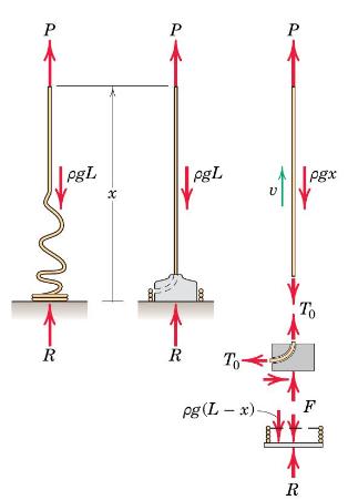
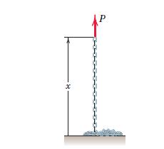
Replace the open-link chain of Sample Problem \(4 / 10\) by a flexible but inextensible rope or bicycle-type chain of length \(L\) and mass \(ho\) per unit length. Determine the force \(P\) required
For each of the following situations, determine whether it is better to use a regular Cartesian, irregular structured, or unstructured grid. Provide arguments supporting your answer. If a grid with
For each of the following situations, determine whether it is better to use a regular Cartesian, irregular structured, or unstructured grid. Provide arguments supporting your answer. If a grid with
Can the numerical instability be avoided by simply using higher precision (larger number of decimal digits) in the computations, thus reducing the round-off error? If not, what would be the effect of
Verify your answers to problem 1 in a simple computational experiment. Use the simple explicit scheme (6.2) to compute the solution of the example problem discussed in the beginning of the chapter.
Consider the heat equation (6.1) with \(a=0.1\) solved in the interval \(0
Answer the same question as in problem 3 but for the simple implicit method.problem 3Consider the heat equation (6.1) with \(a=0.1\) solved in the interval \(0
The heat equation problemis solved using the explicit scheme (6.2). Find the maximum grid steps \(\Delta x\) and \(\Delta t\) at which the expected error of the solution is less than \(\sim
The question is the same as in problem 5 , but now the simple implicit scheme (6.34) is used. Consider two situations.a) The expected error must be less than \(\sim 10^{-4}\) for the entire
Use the Neumann analysis to determine stability properties of the schemeapplied to the linear convection equation \(u_{t}+c u_{x}=0\), where \(c\) is a positive constant. -u At u - u -1 +c = 0 .
Answer the same question as in the previous problem but for the scheme n+1 u+ - u i At un i+1 1 -u-1 +c. = 0. 2Ax
Compare the schemes introduced for the linear convection equation.a) Simple explicit schemes (7.6), (7.7), and (7.8)b) Simple implicit scheme (7.19)c) Leapfrog scheme (7.21)d) Lax-Wendroff scheme
Repeat Problem 7.1 for the following schemes applied to the one-dimensional heat equation.a) Simple explicit scheme \((7.28)\)b) Simple implicit scheme \((7.32)\)c) Crank-Nicolson scheme
Modify the scheme (7.39) for the Burgers equation by changing the central difference approximation of the convective term to the upwind approximation. Assume that \(u\) is always positive. How does
One-dimensional heat equation is solved using the method of lines scheme based on the central difference for space derivative and the Adams-Bashforth scheme (7.43) of the second order \((q=1)\) for
Repeat Problem 7.4 for the scheme based on the Runge-Kutta method of the second order (7.51).
Consider the application of the Thomas algorithm to the simple implicit scheme used to solve the one-dimensional heat equation (see Section 7.5). Modify the algorithm for other sets of boundary
The one-dimensional heat equation is solved on a grid consisting of \(N\) spatial grid points and \(M\) time layers. The boundary conditions are of Dirichlet type. Calculate, in terms of \(N\) and
Apply the Taylor expansion method to prove the order of approximation of two schemes for the linear convection equation.a) Leapfrog scheme (7.21)b) Lax-Wendroff scheme (7.24)
Rewrite the scheme developed in Problem 2 in matrix form. Develop the row equation and expressions for coefficients as in (8.9) and (8.10).Problem 2Develop a finite difference scheme of the second
The two-dimensional heat conduction equation (8.15) is solved in the rectangular domain \(0 \leq x \leq L_{x}, 0 \leq y \leq L_{y}\) with the boundary conditions \(u=0\) at \(x=0, x=L_{x}, y=0,
For the finite difference scheme in Problem 4:a) Write the formulas for the Gauss-Seidel algorithm in terms of the grid point values.b) Prove convergence of the Gauss-Seidel iteration
Derive the expressions for submatrices \(\boldsymbol{B}_{j}, \boldsymbol{D}_{j}, \boldsymbol{A}_{j}\) in the blocktridiagonal form (8.38) of the matrix equation for the five-point discretization
Consider the two-dimensional Poisson equation (8.6) in a rectangular domain \(0 \leq x \leq L_{x}, 0 \leq y \leq L_{y}\). The boundary conditions are\[\frac{\partial u}{\partial x}(0, y)=g_{1}(y),
Write the formulas for the Gauss-Seidel algorithm (similar to (8.57)) for the central difference scheme applied to the three-dimensional Poisson equation (8.14).
Develop a finite difference scheme for the PDE in problem
For a two-dimensional compressible flow with all variables depending on \((x, y, t)\), the equations are written in vector form asRewrite the expressions (2.45) and (2.46) of the vector fields
Can the incompressible flow equations be written in the vector form (9.7)? What are the expressions for the vector fields \(\boldsymbol{U}, \boldsymbol{A}, \boldsymbol{B}\), and \(\boldsymbol{C}\) in
For the two-dimensional system of compressible flow equations in Problem 1, write the complete MacCormack scheme of the second order in space and time. Follow the rules described in Section 9.2.2 to
A three-dimensional flow of air is modeled using the MacCormack scheme. The flow velocity is estimated to be between 1 and \(200 \mathrm{~m} / \mathrm{s}\). The computational grid has \(\Delta
Considering that the Beam-Warming scheme is unconditionally stable, would it be justified to use very large time steps?
For the Beam-Warming scheme, what is the order of error introduced by linearization and by approximate factorization? Does the accuracy of the scheme deteriorate when we use these approximations?
Use matrix algebra to prove that the error introduced by the approximate factorization in the two-dimensional Beam-Warming method is as given by \((9.22)\).
Is the leapfrog scheme (7.21) a good choice for calculation of solutions of the linear convection equation, in which the initial state has a discontinuity, such as in Figure 9.2?
A rectangular bar of dimensions \(L_{x} \times L_{y} \times L_{z}\), constant material properties \(\kappa, ho, C\), and initial temperature \(T_{0}\) is immersed in cold water maintained at constant
Rewrite the finite difference approximations developed in Problem 9.9 for the case when the material properties \(\kappa, ho, C\) are functions of temperature.
Rewrite the finite difference approximations developed in Problem 9 for the situation when the body has the shape of a cylindrical ring of inner and outer radii \(R_{i}\) and \(R_{o}\) and height
How would you proceed with analyzing the heat transfer in Problems \(9-11\) if your interest were only to find the asymptotic equilibrium temperature at \(t \rightarrow \infty\).
Rewrite the approximate factorization method of Section 9.3 .3 for the case of three-dimensional heat conduction equation.
Compare the properties of the approximate factorization method, Crank-Nicolson method (9.35), and simple explicit method (9.33), all applied to solution of two-dimensional heat conduction problems.
Show that the ADI scheme for two-dimensional heat equation can be obtained from the Crank-Nicolson scheme ( 9.35 ) by approximate factorization and that the factorization error is \(O\left((\Delta
The two-dimensional heat equation is solved in a rectangular domain \(0
What is the difference between colocated and staggered grid arrangements? Discuss the comparative advantages of each approach.
If your course involves exercises with a CFD code, study the manual to determine whether the discretization uses staggered or colocated grids. Does the manual say anything about the exact mass
Derive the approximations (10.17) and (10.18) of the pressure gradient terms.
Describe the staggered grid arrangement of finite difference and finite volume structured grids in the three-dimensional case.
Write the finite difference formulas for the nonlinear term of the \(x\)-momentum equation for a two-dimensional flow discretized on a staggered Cartesian uniform grid. The discretization must be of
Write the complete set of formulas for the finite difference discretization of two-dimensional Navier-Stokes equation system for incompressible viscous unsteady flow with zero body forces. Use the
The simple explicit scheme and the projection method (see Section 10.3.1) are applied to compute the flow of an incompressible viscous fluid in a rectangular box \(0
For the flow in Problem 7, write the boundary conditions for pressure when the flow is incompressible and inviscid and there is no body force.
Modify the predictor-corrector formulas (10.27)-(10.30) for the method that uses the second-order Adams-Bashforth time-integration scheme (see Section 7.4.1) instead of the simple explicit scheme.
Show that the decomposition (10.37) of the nonlinear term is correct. Use direct substitution of (10.36) into the expression for one component of vector \(N\).
Consider the explicit, fully implicit, and semi-implicit methods discussed in Section 10.3. Order them by the amount of computations required at every time step. Explain your answer.
Develop the formula (10.43) for the case of the \(x\)-momentum equation of a two-dimensional steady-state incompressible flow discretized on a structured uniform finite difference grid. Use central
Repeat the solution of Problem 12 for the case when the flow is unsteady and the problem is solved using the fully implicit time discretization (the simple implicit scheme).
Compare the four algorithms described in Section 10.4 (SIMPLE, SIMPLER, SIMPLEC, PISO) by the amount of computations required for one iteration. Does the smaller amount necessarily mean smaller time
If your course involves exercises with a CFD code, study the manual to determine which of the projection schemes discussed in Section 10.4 (SIMPLE, SIMPLEC, SIMPLER, PISO) are implemented. Are there
For the following hypothetical CFD tasks, compare the DNS, LES, and RANS approaches. Discuss which of them is feasible and which is likely to produce acceptable accuracy and level of description.a)
For the following hypothetical CFD tasks, compare the DNS, LES, and RANS approaches. Discuss which of them is feasible and which is likely to produce acceptable accuracy and level of description.a)
Does the steady-state formulation of a CFD problem make sense in DNS, LES, or RANS?
DNS of homogeneous turbulence is conducted by the Fourier spectral method (see section 11.2.1) applied to a flow in a periodic box. The expected value of the Reynolds number based on the typical size
Prove that the averaging operations (11.13)-(11.15) are linear and commute with space and time derivatives.
Prove the relations (11.16), (11.18), and (11.21).
\(u(\boldsymbol{x}, t)\) and \(v(\boldsymbol{x}, t)\) are velocity components of a turbulent flow. The RANS averaging \(\langle v(a u+b)angle\) is evaluated, where \(a\) and \(b\) are some constants.
Do the same as in Problem 7 but for the expression \(\left\langle u\left(a u+v^{2}\right)\rightangle\).
If the terms such as those in Problems 7 and 8 appear in the flow equations solved by an RANS method, do they need closure models? Explain your answer.
A steady-state turbulent flow through a long coiled duct is modeled using the standard \(k-\epsilon\) model. Assuming the fluid is incompressible and isothermal, write the full system of equations
For the flow analysis in Problem 10, consider the situation when temperature is not constant. There is an internal heat source with volumetric rate \(Q\). The duct's walls are thermally insulated.
Which of the three RANS model types - algebraic, \(k-\epsilon\) RANS, or \(k-\epsilon\) URANS - would you use in each of the following problems? Assume that the Reynolds number is sufficiently high
If your course involves exercises with CFD software, study the documentation to determine which RANS models are implemented. What approach is taken to the near-wall treatment?
Prove that the LES filtering operation (11.67) is linear and commutes with space and time derivatives. For the space derivatives, consider two cases: a uniform and a nonuniform filter.
What determines the adequate grid step in LES far from the walls?
For a flow past a moving car, would it be correct to apply the LES approach based on the standard Smagorinsky model (see Section 11.4.2) with constant \(C_{S}\) and a uniform finite volume grid
LES is applied to a turbulent flow with convection heat transfer. Apply the filtering operation to (2.29) to derive the LES equation for temperature. Are there any terms that need modeling?
If your course involves exercises with CFD software, study the documentation to determine whether the LES option is implemented. Which closure models are used? What approach is taken to the near-wall
Consider the primitive LES and RANS models, in which the eddy viscosity formulas (11.32) and (11.77) are applied with constant eddy viscosity \(\mu_{t}\). What is the drawback of these models? Should
For each of the flows in Problems 1 and 2, for which an irregular structured grid has been found necessary and possible, suggest a coordinate transformation.
For the coordinate transformation (12.1) and (12.2), derive the formula for \(u_{x y}\).
For the coordinate transformation (12.1) and (12.2), develop the second-order finite difference approximations of \(u_{y}, u_{x x}\), and \(u_{x y}\) at \(\left(\xi_{i}, \eta_{j}\right)\). Apply
If your course involves exercises with a finite volume CFD software, study the software manual to determine which types of cell shapes are available for unstructured grids. Does the software allow
If your course involves exercises with a CFD software equipped with automated grid generation algorithm, try to generate grids for several simple shapes: a pipe of circular cross section, a spherical
In each of the following situations, determine which type of the error (physical model, discretization, iteration, or programming) is most likely responsible for poor performance. In each case,
For the following problems, propose a verification and validation tests of the CFD solution.a) Flow in confluence of two rivers.b) Wind flow around a smokestack of a coal power station and the
Consider the function \(u=\sin x\). Apply the forward difference (4.4), backward difference (4.9), and central difference (4.10) to evaluate the derivative \(d u / d x\) at \(x=1.0\). Use the uniform
In the same way as in Problem 1, compare the performance of the central difference scheme (4.10) and the fourth-order scheme (4.15).Problem 1Consider the function \(u=\sin x\). Apply the forward
Write the schemes similar to (4.4), (4.9), and (4.10) for \(\partial u /\left.\partial y\right|_{i, j}\).
Write the schemes similar to (4.17), (4.18), and (4.19) for \(\partial^{2} u /\left.\partial y^{2}\right|_{i, j}\).
Write the central finite difference formulas of the second order for \(\partial u / \partial x\) and \(\partial^{2} u / \partial x^{2}\) of function \(u(x, y, t)\) at the grid point \(\left(x_{i+1},
Apply the central difference formula (4.10) to approximate the first derivatives of the functions \(u_{1}(x)=\sin (x), u_{2}(x)=\sin (3 x)\), \(u_{3}(x)=\sin (10 x)\) at \(x=0\). Use the uniform grid
Verify the consistency and order of approximation of the schemes (4.13) and (4.14) using Taylor series expansions.
Verify the consistency and order of approximation of the scheme (4.20) using Taylor series expansions.
Verify the statement made in Section 4.2 .7 that the schemeis inconsistent if used with a nonuniform grid. i.j Ui+1j-2uij ui-1,j - (X Xi_1 )
Using the method of Taylor series expansion or the method of polynomial fitting, develop the following finite difference schemes.a) \((4.13)\)b) \((4.17)\)c) \((4.25)\)
Consider the generic transport equation \(\phi_{t}+u \phi_{x}=\mu \phi_{x x}\), where \(u\) is a known function of \(x\) and \(t\) and \(\mu\) is a constant coefficient. Assume that the computational
The Neumann boundary condition \(\partial u / \partial x=a\) at \(x=0\) has to be implemented in a finite difference scheme. The grid is uniform with step \(\Delta x\). Select a finite difference
Consider the PDE problemwhere \(a, b\), and \(\omega\) are constants. Write the full finite difference discretization of the problem on a uniform grid. The discretization must be of the first order
A finite difference scheme was developed to solve the heat equation. Testing in comparison with a known exact solution showed that the error is of the same order of magnitude as the solution itself
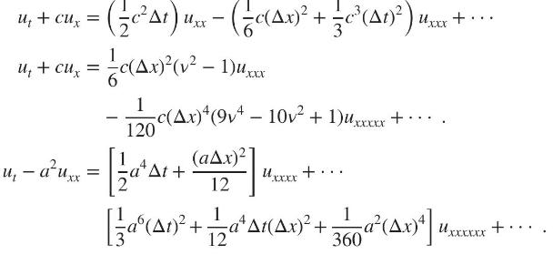
The modified equations of certain finite difference schemes are given below. In each case, determine the order of approximation, and find whether the dominant error is due to numerical dissipation or
Transform the following equations into the integral form similar to (5.1). For each equation, identify, if present, the rate of change term, volumetric source term, convective flux term, and
A finite volume scheme is developed using a two-dimensional structured Cartesian grid with constant steps \(\Delta x\) and \(\Delta y\) (see Figure 5.5a). Write the following approximations using the

Showing 1 - 100 of 2550

1
2
3
4
5
6
7
8
9
10
11
12
13
14
15
Last

Services

Sitemap
Fun
Definitions
Become Tutor
Study Help Categories
Recent Questions
Expert Questions

Company Info

Security
Copyrights
Privacy Policy
Terms & Conditions
SolutionInn Fee
Scholarship

Get In Touch

About Us
Contact Us
Career
Jobs
FAQ
Campus Ambassador

Secure Payment

Download Our App

© 2024 SolutionInn. All Rights Reserved