with steps please

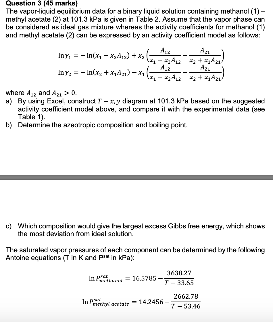
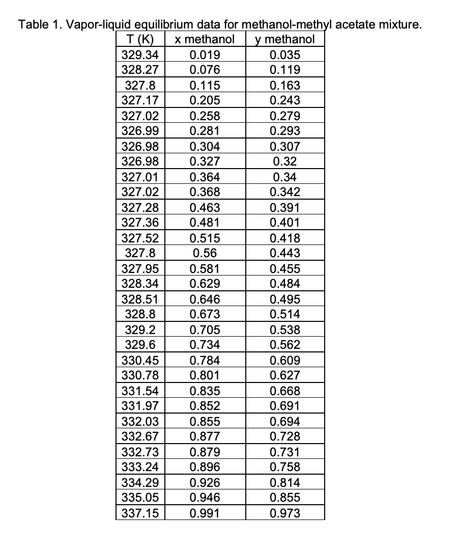
Question 3 (45 marks) The vapor-liquid equilibrium data for a binary liquid solution containing methanol (1) - methyl acetate (2) at 101.3 kPa is given in Table 2. Assume that the vapor phase can be considered as ideal gas mixture whereas the activity coefficients for methanol (1) and methyl acetate (2) can be expressed by an activity coefficient model as follows: A21 A12 In y = In(x1 + x2A12) + x2 \x1 + x2A12 x2 + x1A21) A12 A21 In y2 = - In(x2 + x1A21) X1 \x1 + x2A12 x2 + x1A21 where A12 and A21 > 0. a) By using Excel, construct T x,y diagram at 101.3 kPa based on the suggested activity coefficient model above, and compare it with the experimental data (see Table 1). b) Determine the azeotropic composition and boiling point. c) Which composition would give the largest excess Gibbs free energy, which shows the most deviation from ideal solution. The saturated vapor pressures of each component can be determined by the following Antoine equations (T in K and psat in kPa): In psat methanol = 16.5785 3638.27 T 33.65 2662.78 In psat methyl acetate = 14.2456 T - 53.46 T(K) Table 1. Vapor-liquid equilibrium data for methanol-methyl acetate mixture. x methanol y methanol 329.34 0.019 0.035 328.27 0.076 0.119 327.8 0.115 0.163 327.17 0.205 0.243 327.02 0.258 0.279 326.99 0.281 0.293 326.98 0.304 0.307 326.98 0.327 0.32 327.01 0.364 0.34 327.02 0.368 0.342 327.28 0.463 0.391 327.36 0.481 0.401 327.52 0.515 0.418 327.8 0.56 0.443 327.95 0.581 0.455 328.34 0.629 0.484 328.51 0.646 0.495 328.8 0.673 0.514 329.2 0.705 0.538 329.6 0.734 0.562 330.45 0.784 0.609 330.78 0.801 0.627 331.54 0.835 0.668 331.97 0.852 0.691 332.03 0.855 0.694 332.67 0.877 0.728 332.73 0.879 0.731 333.24 0.896 0.758 334.29 0.926 0.814 335.05 0.946 0.855 337.15 0.991 0.973 Question 3 (45 marks) The vapor-liquid equilibrium data for a binary liquid solution containing methanol (1) - methyl acetate (2) at 101.3 kPa is given in Table 2. Assume that the vapor phase can be considered as ideal gas mixture whereas the activity coefficients for methanol (1) and methyl acetate (2) can be expressed by an activity coefficient model as follows: A21 A12 In y = In(x1 + x2A12) + x2 \x1 + x2A12 x2 + x1A21) A12 A21 In y2 = - In(x2 + x1A21) X1 \x1 + x2A12 x2 + x1A21 where A12 and A21 > 0. a) By using Excel, construct T x,y diagram at 101.3 kPa based on the suggested activity coefficient model above, and compare it with the experimental data (see Table 1). b) Determine the azeotropic composition and boiling point. c) Which composition would give the largest excess Gibbs free energy, which shows the most deviation from ideal solution. The saturated vapor pressures of each component can be determined by the following Antoine equations (T in K and psat in kPa): In psat methanol = 16.5785 3638.27 T 33.65 2662.78 In psat methyl acetate = 14.2456 T - 53.46 T(K) Table 1. Vapor-liquid equilibrium data for methanol-methyl acetate mixture. x methanol y methanol 329.34 0.019 0.035 328.27 0.076 0.119 327.8 0.115 0.163 327.17 0.205 0.243 327.02 0.258 0.279 326.99 0.281 0.293 326.98 0.304 0.307 326.98 0.327 0.32 327.01 0.364 0.34 327.02 0.368 0.342 327.28 0.463 0.391 327.36 0.481 0.401 327.52 0.515 0.418 327.8 0.56 0.443 327.95 0.581 0.455 328.34 0.629 0.484 328.51 0.646 0.495 328.8 0.673 0.514 329.2 0.705 0.538 329.6 0.734 0.562 330.45 0.784 0.609 330.78 0.801 0.627 331.54 0.835 0.668 331.97 0.852 0.691 332.03 0.855 0.694 332.67 0.877 0.728 332.73 0.879 0.731 333.24 0.896 0.758 334.29 0.926 0.814 335.05 0.946 0.855 337.15 0.991 0.973