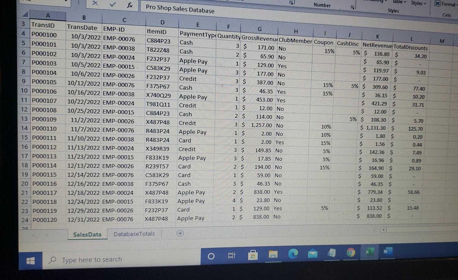
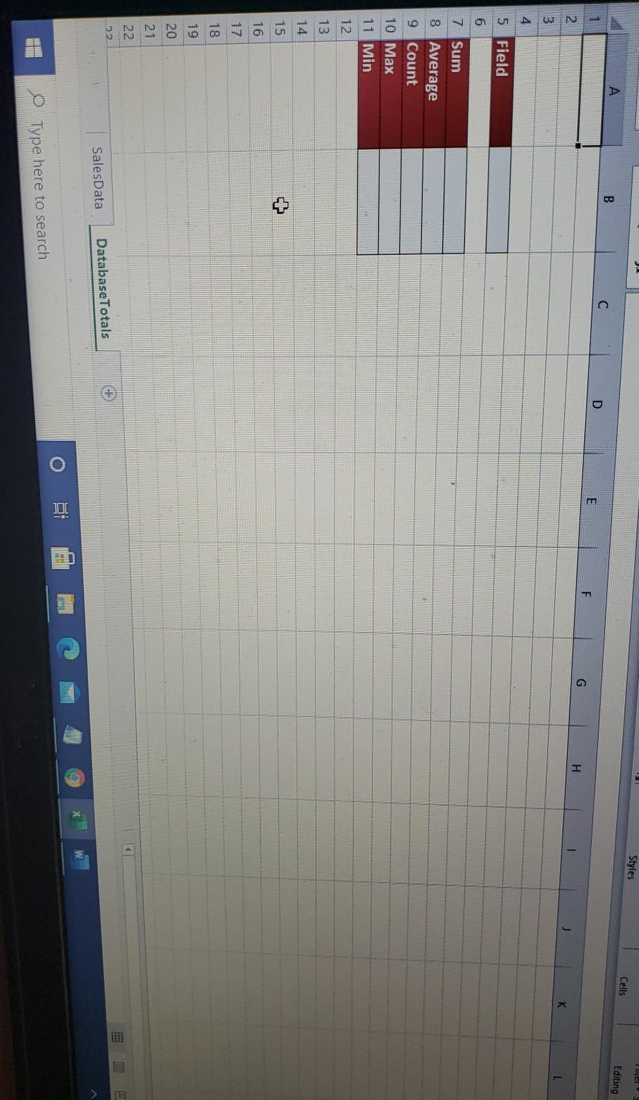
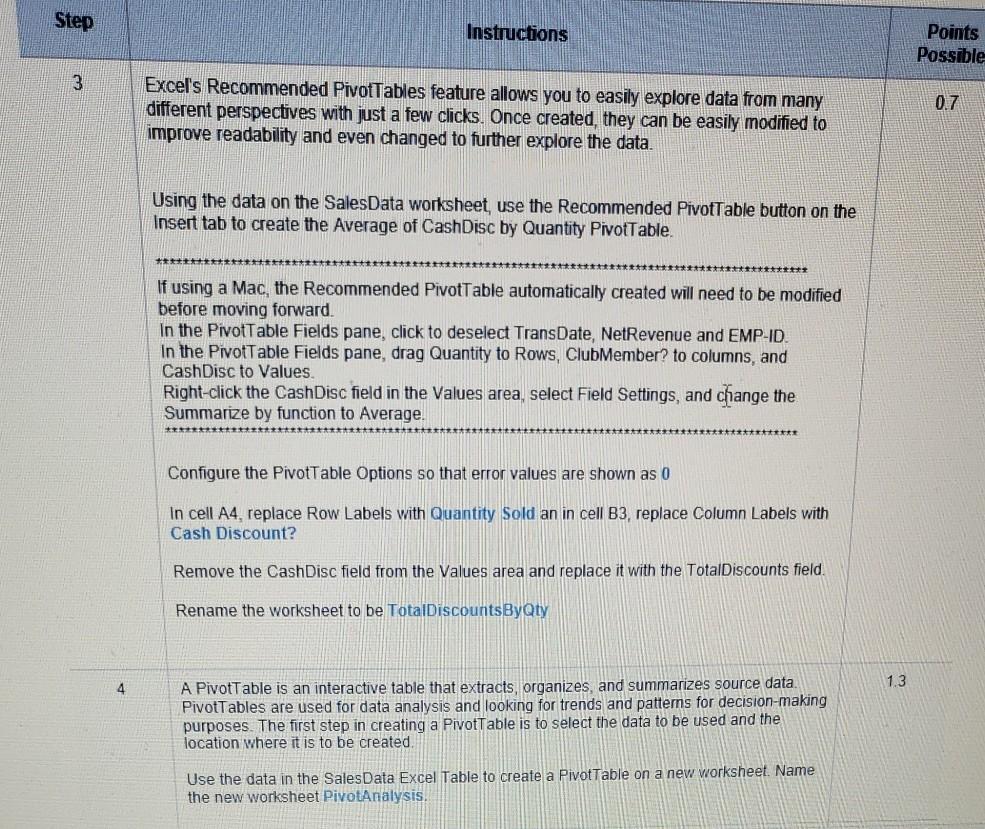
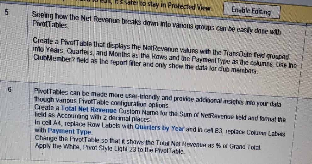
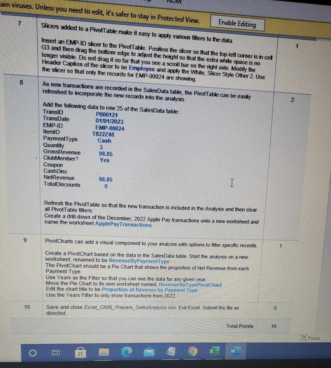
43 AaBbCcDc AaBbc AaBbCc) AaBbCcDd AaBbCcDd Emphasis Heading 1 Heading 2 11 Normal 1 Normal ... Paragraph Styles Instructions Points Possible exercise begins on page 343 of your text. Start Excel. Download and open the file d Excel_Ch06_Prepare_SalesAnalysis.xlsx. Grader has automatically added your last to the beginning of the filename. Save the file to the location where you are storing your 0 base functions allow for the user to specify criteria in one or more fields to explore the with ease. When this is done, all the criteria must be evaluated to TRUE for the record to cluded in the calculation. Using a table for the Excel Database allows you to add new ds to the database easily and any database functions used on the table will automatically ce 1.5 e SalesRata worksheet, convert the plain data set to an Excel table. Name the Excel Sales Data and then create a named range, Sales Database for all of the data in the including the column headings the column headings from the SalesData table and paste them on the Database Totals sheet, starting in cell A1 to setup the criteria area of for use in the Database functions. e Database Totals worksheet in cell B5, type NetRevenue for the field name that will be in the database functions Is B7 B11, use the appropriate Database function to calculate the sum average, count and min of the NetRevenue field using the range A1 L2 as the criteria. all database functions have been created, use the criteria area to limit the calculations to e records with transaction dates after 11/15/2022 and with Apple Pay as the payment od. ly, change the field being used in the calculations from NetRevenue to Jataj Discounts. Focus home end prt se 8. Emphasis Heading 1 Heading 2 Paragraph 1 Normal Normal ... Styles Instructions Poin Possi I's Recommended Pivot Tables feature allows you to easily explore data from many ent perspectives with just a few clicks. Once created, they can be easily modified to ve readability and even changed to further explore the data 0.7 the data on the SalesRata worksheet, use the Recommended PivotTable button on the t tab to create the Average of Cash Disc by Quantity PivotTable tttttttttt ng a Mac, the Recommended PivotTable automatically created will need to be modified re moving forward. PivotTable Fields pane, click to deselect Trans Rate NetRevenue and EMP-ID. e PivotTable Fields pane, drag Quantity to Rows, Club Member? to columns and Disc to Values t-click the CashDisc field in the Values area, select Field Settings, and change the marize by function to Average ********** figure the PivotTable Options so that error values are shown as 0 Terace ell A4, replace Row Labels with Quantity Sold an in cell B3, reprace Column Labels with h Discount? nove the Cash Disc field from the Values area and replace it with the TotalDiscounts field name the worksheet to be TotalDiscountsByQty. 1.3 ivotTable is an interactive table that extracts, organizes and summarizes source data Tables are used for data analysis and looking for trends and pattems for decision-making poses. The first step in creating a PivotTable is to select the data to be used and the ation where it is to be created Focu home end presc 8 hU6_Prepare_PartB_Sales_Analysis_Instructions - Read-Only - Word Mailings Review View Help RCM AaBbCcDc AaBbc AaBbCc AaBbCcDd AaBBCCD- Emphasis Heading 1 Heading 2 I Normal Normal.. Paragraph Styles A Pivot Table is an interactive table that extracts, organizes, and summarizes source data. PivotTables are used for data analysis and looking for trends and pattems for decision-making purposes. The first step in creating a PivotTable is to select the data to be used and the location where it is to be created. 1 Use the data in the Sales Data Excel Table to create a PivotTable on a new worksheet Name the new worksheet PivotAnalysis Seeing how the Net Revenue breaks down into various groups can be easily done with PivotTables 1.5 Create a PivotTable that displays the NetRevenue values with the TransRate field grouped into Years, Quarters, and Months as the Rows and the Payment Tyre as the columns. Use the Club Member? field as the report filter and only show the data for club members. 1 PivotTables can be made more user-friendly and provide additional insights into your data though various PivotTable configuration options. Create a Total Net Revenue Custom Name for the Sum of NetRevenue field and format the field as Accounting with 2 decimal places. In cell A4, replace Row Labels with Quarters by Year and in cell B3, replace Column Labels with Payment Type. Change the PivotTable so that it shows the Total Net Revenue as % of Grand Total Apply the White, Pivot Style Light 23 to the PivotTable. VOLEN CROGL Prepare Sales Analysis Part B 11 . inse home end prt sc FIO Slicers added to a PivotTable make it easy to apply various filters to the data PC nsert an EMP-ID slicer to the PivotTable. Position the slicer so that the top-left corner is in cell 53 and then drag the bottom edge to adjust the height so that the extra white space is no Onger visible. Do not drag it so far that you see a scroll bar on the right side. Modify the Header Caption of the slicer to be Employee and apply the White, Slicer Style Other 2. Use he slicer so that only the records for EMP-00024 are showing As new transactions are recorded in the SalesRata table, the PivotTable can be easily efreshed to incorporate the new records into the analysis. Add the following data to row 25 of the SalesRata table Transla P000121 Translate 01/01/2023 EMP-ID EMP-00024 Itemid T822748 PaymentType Cash Quantity 3 GrossRevenue 98.85 ClubMember? Coupon CashDisc NetRevenue 98.85 TotalDiscounts 0 Yes Refresh the Pivottable so that the new transaction is included in the Analysis and then clear all PivotTable filters Create a drill-down of the December, 2022 Apple Pay transactions onto a new worksheet and name the worksheet AnglePaxtiansactions, PivoiCharts can add a visual component to your analysis with options to filter specific records 1 Create a PivotChart based on the data in the Sales Data table Start the analysis on a new prt sc home end 8 T View Help RCM E ALT AaBbCcDc AaBbc AaBb c Aabbccd AaE Emphasis Heading 1 Heading 2 11 Normal Ne Paragraph Cash Disc NetRevenue TotalDiscounts Styles 98.85 0 Refresh the Pivot Table so that the new transaction is included in the Analysis and then clear all Pivot Table filters Create a drill-down of the December 2022 Apple Pay transactions onto a new worksheet and name the worksheet ApplePayTransactions, 9 Pixetsbarts can add a visual component to your analysis with options to filter specific records. Create a PivotChart based on the data in the Sales Data table. Start the analysis on a new worksheet, renamed to be RevenueByPaymentType The PivotChart should be a Pie Chart that shows the proportion of Net Revenue from each Payment Type Use Years as the Filter so that you can see the data for any given year. Move the Pie Chart to its own worksheet named, RexenueBxIynePixotchart Edit the chart title to be Proportion of Revenue by Payment Type Use the Years Filter to only show transactions from 2022 10 Save and close Excel_Ch06_Prepare_Sales Analysis.x/sx Exit Excel. Submit the file as directed Total Points 1 home end prt sc X lable Number Styles Pro Shop Sales Database Format Styles A Cells M 3 TransID 4 P000100 5 PO00101 6 P000102 7 P000103 8 P000104 D ItemID C884P23 T822748 F232P37 C583K29 F232P37 F375P67 X740029 T981011 9 P000105 10 P000106 11 P000107 12 P000108 13 P000109 C884P23 B c TransDate EMP-ID 10/3/2022 EMP-00076 10/3/2022 EMP-00038 10/3/2022 EMP-00024 10/5/2022 EMP-00015 10/6/2022 EMP-00026 10/12/2022 EMP-00076 10/16/2022 EMP-00038 10/22/2022 EMP-00024 10/25/2022 EMP-00015 11/2/2022 EMP-00026 11/7/2022 EMP-00076 11/10/2022 EMP-00038 11/13/2022 EMP-00024 11/23/2022 EMP-00015 12/13/2022 EMP-00026 12/14/2022 EMP-00076 12/16/2022 EMP-00038 12/18/2022 EMP-00024 12/24/2022 EMP-00015 12/29/2022 EMP-00026 12/31/2022 EMP-00076 E F G H PaymentType Quantity GrossRevenue Club Member Coupon CashDisc NetRevenue TotalDiscounts J K Cash 3 $ 171.00 No Cash 15% 5% $ 136.80 $ 2 $ 65.90 No 34.20 Apple Pay $ 65.90 $ 1 $ 129.00 Yes Apple Pay $ 119.97 $ 9.03 3 $ 177.00 No Credit $ 177.00 $ 3 $ 387.00 No 15% 5% $ 309.60 $ 77.40 Cash 3 $ 46.35 Yes 15% $ 36.15 $ 10.20 Apple Pay 1 $ 453.00 Yes $ 421.29 $ 31.71 Credit 1 S 12.00 No $ 12.00 $ Cash 2 $ 114.00 No 5% $ 108.30 $ 5.70 Credit 3 $ 1,257.00 No 10% $ 1,131.30 $ 125.70 Apple Pay 1$ 2.00 No 10% $ 1.80 $ 0.20 Card 1 $ 2.00 Yes 15% $ 1.56 $ 0.44 Credit 3 S 149.85 No 5% $ 142.36 $ 7.49 Apple Pay 3 $ 17.85 No 5% $ 16.96 $ 0.89 Card 2 $ 194.00 No 15% $ 164.90 $ 29.10 Card 1 $ 59.00 No S 59.00 $ Cash 3 S 46.35 No S 46.35 $ 2 $ 838.00 Yes $ Apple Pay 779.34 $ 58.66 4 S 23.80 No $ 23.80 $ Apple Pay 5% 1 S 129.00 Yes S 15.48 113.52 $ Card $ 838.00 S 2 S 838.00 No Apple Pay X487P48 R483P24 14 P000110 15 P000111 R483P24 16 P000112 17 P000113 X349R39 F833K19 R239T57 18 P000114 19 P000115 20 P000116 C583K29 F375P67 X487248 F833619 21 PO00117 22 PO00118 23 P000119 24 P000120 F232P37 X487248 Sales Data Database Totals Type here to search el Styles Cells A Editing B. 1 D El F G 2 H L 3 4 5 Field 6 7 Sum 8 Average 9 Count 10 Max 11 Min 12 13 14 15 16 17 18 19 20 22 Sales Data Database Totals X II o Type here to search les from the Internet can contain viruses. Unless you need to edit, it's safer to stay in Protected View. Enable Editing Grader-Instructions Excel 2019 Project YO19_Excel_Ch06_Prepare_PartB_Sales_Analysis Project Description: Aleeta Herriott, manager of the Red Bluff Pro Shop, would like to develop a marketing strategy for increasing pro shop patronage. She has requested data about the pro shop sales over the past several years. She needs to be able to work with the data to understand the current patronage, such as where the patrons were from, what kind of items they purchased, how much money they spent, and so forth. Exploring the data is key in determining the marketing strategy because it helps her learn about customer preferences. After analyzing the data, Aleeta will present her ideas to the board of directors. Steps to Perform: Points Possible Step Instructions 0 1 This exercise begins on page 343 of your text. Start Excel. Download and open the file named Excel_Ch06_Prepare_SalesAnalysis.xlsx Grader has automatically added your last name to the beginning of the filename. Save the file to the location where you are storing your files 1.5 2. Database functions allow for the user to specify criteria in one or more fields to explore the data with ease. When this is done, all the criteria must be evaluated to TRUE for the record to be included in the calculation. Using a table for the Excel Database allows you to add new records to the database easily and any database functions used on the table will automatically update On the Sales Data worksheet, convert the plain data set to an Excel table. Name the Excel table, Sales Data and then create a named range, Sales Database, for all of the data in the table, including the column headings Copy the column headings from the Sales Data table and paste them on the Database Totals worksheet, starting in cell A1 to setup the criteria area of for use in the Database functions. On the Database Totals worksheet in cell B5, type NetRevenue for the field name that will be used in the database functions Focus In cells B7:B11, use the appropriate Database function to calculate the sum, average, count, max, and min of the NetRevenue field using the range A1 L2 as the criteria. X W 1 of 1716 words O In cells B7:B11, use the appropriate Database function to calculate the sum, average, count, max, and min of the NetRevenue field using the range A1L2 as the criteria. Once all database functions have been created, use the criteria area to limit the calculations to those records with transaction dates after 11/15/2022 and with Apple Pay as the payment method. Finally, change the field being used in the calculations from NetRevenue to TotalDiscounts. Step Instructions Points Possible 3 Excel's Recommended PivotTables feature allows you to easily explore data from many different perspectives with just a few clicks. Once created, they can be easily modified to improve readability and even changed to further explore the data. 0.7 Using the data on the SalesData worksheet, use the Recommended PivotTable button on the Insert tab to create the Average of CashDisc by Quantity PivotTable. ttt++ tttttttttttttttttttttttttttt If using a Mac, the Recommended PivotTable automatically created will need to be modified before moving forward. In the Pivot Table Fields pane, click to deselect TransDate, NetRevenue and EMP-ID. In the Pivot Table Fields pane, drag Quantity to Rows, Club Member? to columns, and CashDisc to Values. Right-click the CashDisc field in the Values area, select Field Settings, and change the Summarize by function to Average. *** Configure the PivotTable Options so that error values are shown as 0 In cell A4, replace Row Labels with Quantity Sold an in cell B3, replace Column Labels with Cash Discount? Remove the CashDisc field from the Values area and replace it with the TotalDiscounts field. Rename the worksheet to be TotalDiscountsByQty 1.3 4 A PivotTable is an interactive table that extracts, organizes, and summarizes source data. PivotTables are used for data analysis and looking for trends and patterns for decision-making purposes. The first step in creating a Pivot Table is to select the data to be used and the location where it is to be created Use the data in the Sales Data Excel Table to create a Pivot Table on a new worksheet. Name the new worksheet PivotAnalysis, It's safer to stay in Protected View. Enable Editing 5 Seeing how the Net Revenue breaks down into various groups can be easily done with PivotTables Create a PivotTable that displays the NetRevenue values with the TransDate field grouped into Years, Quarters, and Months as the Rows and the PaymentType as the columns. Use the Club Member? field as the report filter and only show the data for dub members. 6 PivotTables can be made more user-friendly and provide additional insights into your data though various PivotTable configuration options. Create a Total Net Revenue Custom Name for the Sum of NetRevenue field and format the field as Accounting with 2 decimal places. In cell A4, replace Row Labels with Quarters by Year and in cell B3, replace Column Labels with Payment Type. Change the PivotTable so that it shows the Total Net Revenue as % of Grand Total. Apply the White, Pivot Style Light 23 to the PivotTable. Eain viruses. Unless you need to edit, it's safer to stay in Protected View. IV 7 Enable Editing Slicers added to a Pivot Table make it easy to apply various fifers to the data. 1 Insert an EMP-D slicer to the Pivot Table. Position the slicer so that the top-left comer is in cel G3 and then drag the bottom edge to adjust the height so that the extra white space is no longer visible. Do not drag it so far that you see a scroll bar on the right side. Modify the Header Caption of the slicer to be Employee and apply the White, Slicer Style Other 2. Use the slicer so that only the records for EMP-00024 are showing 8 As new transactions are recorded in the Sales Data table, the PivotTable can be easily refreshed to incorporate the new records into the analysis. 2 Add the following data to row 25 of the SalesData table: TransID P000121 TransDate 01/01/2023 EMP-D EMP-00024 ItemID T822748 PaymentType Cash Quantity 3 GrossRevenue 98.85 Club Member? Yes Coupon Cash Disc NetRevenue 98.85 TotalDiscounts 0 Refresh the PivotTable so that the new transaction is included in the Analysis and then clear all Pivot Table filters. Create a drill-down of the December, 2022 Apple Pay transactions onto a new worksheet and name the worksheet Apple PayTransactions. 9 PivotCharts can add a visual component to your analysis with options to filter specific records. 1 Create a PivotChart based on the data in the Sales Data table Start the analysis on a new worksheet, renamed to be Revenue ByPaymentType The PivotChart should be a Pie Chart that shows the proportion of Net Revenue from each Payment Type Use Years as the Filter so that you can see the data for any given year. Move the Pie Chart to its own worksheet named. RevenueByTypePivotChart Edit the chart title to be Proportion of Revenue by Payment Type Use the Years Filter to only show transactions from 2022 10 Save and close Excel_Ch06_Prepare_SalesAnalysis xlsx. Exit Excel. Submit the file as directed 0 Total Points 10 Focus A 43 AaBbCcDc AaBbc AaBbCc) AaBbCcDd AaBbCcDd Emphasis Heading 1 Heading 2 11 Normal 1 Normal ... Paragraph Styles Instructions Points Possible exercise begins on page 343 of your text. Start Excel. Download and open the file d Excel_Ch06_Prepare_SalesAnalysis.xlsx. Grader has automatically added your last to the beginning of the filename. Save the file to the location where you are storing your 0 base functions allow for the user to specify criteria in one or more fields to explore the with ease. When this is done, all the criteria must be evaluated to TRUE for the record to cluded in the calculation. Using a table for the Excel Database allows you to add new ds to the database easily and any database functions used on the table will automatically ce 1.5 e SalesRata worksheet, convert the plain data set to an Excel table. Name the Excel Sales Data and then create a named range, Sales Database for all of the data in the including the column headings the column headings from the SalesData table and paste them on the Database Totals sheet, starting in cell A1 to setup the criteria area of for use in the Database functions. e Database Totals worksheet in cell B5, type NetRevenue for the field name that will be in the database functions Is B7 B11, use the appropriate Database function to calculate the sum average, count and min of the NetRevenue field using the range A1 L2 as the criteria. all database functions have been created, use the criteria area to limit the calculations to e records with transaction dates after 11/15/2022 and with Apple Pay as the payment od. ly, change the field being used in the calculations from NetRevenue to Jataj Discounts. Focus home end prt se 8. Emphasis Heading 1 Heading 2 Paragraph 1 Normal Normal ... Styles Instructions Poin Possi I's Recommended Pivot Tables feature allows you to easily explore data from many ent perspectives with just a few clicks. Once created, they can be easily modified to ve readability and even changed to further explore the data 0.7 the data on the SalesRata worksheet, use the Recommended PivotTable button on the t tab to create the Average of Cash Disc by Quantity PivotTable tttttttttt ng a Mac, the Recommended PivotTable automatically created will need to be modified re moving forward. PivotTable Fields pane, click to deselect Trans Rate NetRevenue and EMP-ID. e PivotTable Fields pane, drag Quantity to Rows, Club Member? to columns and Disc to Values t-click the CashDisc field in the Values area, select Field Settings, and change the marize by function to Average ********** figure the PivotTable Options so that error values are shown as 0 Terace ell A4, replace Row Labels with Quantity Sold an in cell B3, reprace Column Labels with h Discount? nove the Cash Disc field from the Values area and replace it with the TotalDiscounts field name the worksheet to be TotalDiscountsByQty. 1.3 ivotTable is an interactive table that extracts, organizes and summarizes source data Tables are used for data analysis and looking for trends and pattems for decision-making poses. The first step in creating a PivotTable is to select the data to be used and the ation where it is to be created Focu home end presc 8 hU6_Prepare_PartB_Sales_Analysis_Instructions - Read-Only - Word Mailings Review View Help RCM AaBbCcDc AaBbc AaBbCc AaBbCcDd AaBBCCD- Emphasis Heading 1 Heading 2 I Normal Normal.. Paragraph Styles A Pivot Table is an interactive table that extracts, organizes, and summarizes source data. PivotTables are used for data analysis and looking for trends and pattems for decision-making purposes. The first step in creating a PivotTable is to select the data to be used and the location where it is to be created. 1 Use the data in the Sales Data Excel Table to create a PivotTable on a new worksheet Name the new worksheet PivotAnalysis Seeing how the Net Revenue breaks down into various groups can be easily done with PivotTables 1.5 Create a PivotTable that displays the NetRevenue values with the TransRate field grouped into Years, Quarters, and Months as the Rows and the Payment Tyre as the columns. Use the Club Member? field as the report filter and only show the data for club members. 1 PivotTables can be made more user-friendly and provide additional insights into your data though various PivotTable configuration options. Create a Total Net Revenue Custom Name for the Sum of NetRevenue field and format the field as Accounting with 2 decimal places. In cell A4, replace Row Labels with Quarters by Year and in cell B3, replace Column Labels with Payment Type. Change the PivotTable so that it shows the Total Net Revenue as % of Grand Total Apply the White, Pivot Style Light 23 to the PivotTable. VOLEN CROGL Prepare Sales Analysis Part B 11 . inse home end prt sc FIO Slicers added to a PivotTable make it easy to apply various filters to the data PC nsert an EMP-ID slicer to the PivotTable. Position the slicer so that the top-left corner is in cell 53 and then drag the bottom edge to adjust the height so that the extra white space is no Onger visible. Do not drag it so far that you see a scroll bar on the right side. Modify the Header Caption of the slicer to be Employee and apply the White, Slicer Style Other 2. Use he slicer so that only the records for EMP-00024 are showing As new transactions are recorded in the SalesRata table, the PivotTable can be easily efreshed to incorporate the new records into the analysis. Add the following data to row 25 of the SalesRata table Transla P000121 Translate 01/01/2023 EMP-ID EMP-00024 Itemid T822748 PaymentType Cash Quantity 3 GrossRevenue 98.85 ClubMember? Coupon CashDisc NetRevenue 98.85 TotalDiscounts 0 Yes Refresh the Pivottable so that the new transaction is included in the Analysis and then clear all PivotTable filters Create a drill-down of the December, 2022 Apple Pay transactions onto a new worksheet and name the worksheet AnglePaxtiansactions, PivoiCharts can add a visual component to your analysis with options to filter specific records 1 Create a PivotChart based on the data in the Sales Data table Start the analysis on a new prt sc home end 8 T View Help RCM E ALT AaBbCcDc AaBbc AaBb c Aabbccd AaE Emphasis Heading 1 Heading 2 11 Normal Ne Paragraph Cash Disc NetRevenue TotalDiscounts Styles 98.85 0 Refresh the Pivot Table so that the new transaction is included in the Analysis and then clear all Pivot Table filters Create a drill-down of the December 2022 Apple Pay transactions onto a new worksheet and name the worksheet ApplePayTransactions, 9 Pixetsbarts can add a visual component to your analysis with options to filter specific records. Create a PivotChart based on the data in the Sales Data table. Start the analysis on a new worksheet, renamed to be RevenueByPaymentType The PivotChart should be a Pie Chart that shows the proportion of Net Revenue from each Payment Type Use Years as the Filter so that you can see the data for any given year. Move the Pie Chart to its own worksheet named, RexenueBxIynePixotchart Edit the chart title to be Proportion of Revenue by Payment Type Use the Years Filter to only show transactions from 2022 10 Save and close Excel_Ch06_Prepare_Sales Analysis.x/sx Exit Excel. Submit the file as directed Total Points 1 home end prt sc X lable Number Styles Pro Shop Sales Database Format Styles A Cells M 3 TransID 4 P000100 5 PO00101 6 P000102 7 P000103 8 P000104 D ItemID C884P23 T822748 F232P37 C583K29 F232P37 F375P67 X740029 T981011 9 P000105 10 P000106 11 P000107 12 P000108 13 P000109 C884P23 B c TransDate EMP-ID 10/3/2022 EMP-00076 10/3/2022 EMP-00038 10/3/2022 EMP-00024 10/5/2022 EMP-00015 10/6/2022 EMP-00026 10/12/2022 EMP-00076 10/16/2022 EMP-00038 10/22/2022 EMP-00024 10/25/2022 EMP-00015 11/2/2022 EMP-00026 11/7/2022 EMP-00076 11/10/2022 EMP-00038 11/13/2022 EMP-00024 11/23/2022 EMP-00015 12/13/2022 EMP-00026 12/14/2022 EMP-00076 12/16/2022 EMP-00038 12/18/2022 EMP-00024 12/24/2022 EMP-00015 12/29/2022 EMP-00026 12/31/2022 EMP-00076 E F G H PaymentType Quantity GrossRevenue Club Member Coupon CashDisc NetRevenue TotalDiscounts J K Cash 3 $ 171.00 No Cash 15% 5% $ 136.80 $ 2 $ 65.90 No 34.20 Apple Pay $ 65.90 $ 1 $ 129.00 Yes Apple Pay $ 119.97 $ 9.03 3 $ 177.00 No Credit $ 177.00 $ 3 $ 387.00 No 15% 5% $ 309.60 $ 77.40 Cash 3 $ 46.35 Yes 15% $ 36.15 $ 10.20 Apple Pay 1 $ 453.00 Yes $ 421.29 $ 31.71 Credit 1 S 12.00 No $ 12.00 $ Cash 2 $ 114.00 No 5% $ 108.30 $ 5.70 Credit 3 $ 1,257.00 No 10% $ 1,131.30 $ 125.70 Apple Pay 1$ 2.00 No 10% $ 1.80 $ 0.20 Card 1 $ 2.00 Yes 15% $ 1.56 $ 0.44 Credit 3 S 149.85 No 5% $ 142.36 $ 7.49 Apple Pay 3 $ 17.85 No 5% $ 16.96 $ 0.89 Card 2 $ 194.00 No 15% $ 164.90 $ 29.10 Card 1 $ 59.00 No S 59.00 $ Cash 3 S 46.35 No S 46.35 $ 2 $ 838.00 Yes $ Apple Pay 779.34 $ 58.66 4 S 23.80 No $ 23.80 $ Apple Pay 5% 1 S 129.00 Yes S 15.48 113.52 $ Card $ 838.00 S 2 S 838.00 No Apple Pay X487P48 R483P24 14 P000110 15 P000111 R483P24 16 P000112 17 P000113 X349R39 F833K19 R239T57 18 P000114 19 P000115 20 P000116 C583K29 F375P67 X487248 F833619 21 PO00117 22 PO00118 23 P000119 24 P000120 F232P37 X487248 Sales Data Database Totals Type here to search el Styles Cells A Editing B. 1 D El F G 2 H L 3 4 5 Field 6 7 Sum 8 Average 9 Count 10 Max 11 Min 12 13 14 15 16 17 18 19 20 22 Sales Data Database Totals X II o Type here to search les from the Internet can contain viruses. Unless you need to edit, it's safer to stay in Protected View. Enable Editing Grader-Instructions Excel 2019 Project YO19_Excel_Ch06_Prepare_PartB_Sales_Analysis Project Description: Aleeta Herriott, manager of the Red Bluff Pro Shop, would like to develop a marketing strategy for increasing pro shop patronage. She has requested data about the pro shop sales over the past several years. She needs to be able to work with the data to understand the current patronage, such as where the patrons were from, what kind of items they purchased, how much money they spent, and so forth. Exploring the data is key in determining the marketing strategy because it helps her learn about customer preferences. After analyzing the data, Aleeta will present her ideas to the board of directors. Steps to Perform: Points Possible Step Instructions 0 1 This exercise begins on page 343 of your text. Start Excel. Download and open the file named Excel_Ch06_Prepare_SalesAnalysis.xlsx Grader has automatically added your last name to the beginning of the filename. Save the file to the location where you are storing your files 1.5 2. Database functions allow for the user to specify criteria in one or more fields to explore the data with ease. When this is done, all the criteria must be evaluated to TRUE for the record to be included in the calculation. Using a table for the Excel Database allows you to add new records to the database easily and any database functions used on the table will automatically update On the Sales Data worksheet, convert the plain data set to an Excel table. Name the Excel table, Sales Data and then create a named range, Sales Database, for all of the data in the table, including the column headings Copy the column headings from the Sales Data table and paste them on the Database Totals worksheet, starting in cell A1 to setup the criteria area of for use in the Database functions. On the Database Totals worksheet in cell B5, type NetRevenue for the field name that will be used in the database functions Focus In cells B7:B11, use the appropriate Database function to calculate the sum, average, count, max, and min of the NetRevenue field using the range A1 L2 as the criteria. X W 1 of 1716 words O In cells B7:B11, use the appropriate Database function to calculate the sum, average, count, max, and min of the NetRevenue field using the range A1L2 as the criteria. Once all database functions have been created, use the criteria area to limit the calculations to those records with transaction dates after 11/15/2022 and with Apple Pay as the payment method. Finally, change the field being used in the calculations from NetRevenue to TotalDiscounts. Step Instructions Points Possible 3 Excel's Recommended PivotTables feature allows you to easily explore data from many different perspectives with just a few clicks. Once created, they can be easily modified to improve readability and even changed to further explore the data. 0.7 Using the data on the SalesData worksheet, use the Recommended PivotTable button on the Insert tab to create the Average of CashDisc by Quantity PivotTable. ttt++ tttttttttttttttttttttttttttt If using a Mac, the Recommended PivotTable automatically created will need to be modified before moving forward. In the Pivot Table Fields pane, click to deselect TransDate, NetRevenue and EMP-ID. In the Pivot Table Fields pane, drag Quantity to Rows, Club Member? to columns, and CashDisc to Values. Right-click the CashDisc field in the Values area, select Field Settings, and change the Summarize by function to Average. *** Configure the PivotTable Options so that error values are shown as 0 In cell A4, replace Row Labels with Quantity Sold an in cell B3, replace Column Labels with Cash Discount? Remove the CashDisc field from the Values area and replace it with the TotalDiscounts field. Rename the worksheet to be TotalDiscountsByQty 1.3 4 A PivotTable is an interactive table that extracts, organizes, and summarizes source data. PivotTables are used for data analysis and looking for trends and patterns for decision-making purposes. The first step in creating a Pivot Table is to select the data to be used and the location where it is to be created Use the data in the Sales Data Excel Table to create a Pivot Table on a new worksheet. Name the new worksheet PivotAnalysis, It's safer to stay in Protected View. Enable Editing 5 Seeing how the Net Revenue breaks down into various groups can be easily done with PivotTables Create a PivotTable that displays the NetRevenue values with the TransDate field grouped into Years, Quarters, and Months as the Rows and the PaymentType as the columns. Use the Club Member? field as the report filter and only show the data for dub members. 6 PivotTables can be made more user-friendly and provide additional insights into your data though various PivotTable configuration options. Create a Total Net Revenue Custom Name for the Sum of NetRevenue field and format the field as Accounting with 2 decimal places. In cell A4, replace Row Labels with Quarters by Year and in cell B3, replace Column Labels with Payment Type. Change the PivotTable so that it shows the Total Net Revenue as % of Grand Total. Apply the White, Pivot Style Light 23 to the PivotTable. Eain viruses. Unless you need to edit, it's safer to stay in Protected View. IV 7 Enable Editing Slicers added to a Pivot Table make it easy to apply various fifers to the data. 1 Insert an EMP-D slicer to the Pivot Table. Position the slicer so that the top-left comer is in cel G3 and then drag the bottom edge to adjust the height so that the extra white space is no longer visible. Do not drag it so far that you see a scroll bar on the right side. Modify the Header Caption of the slicer to be Employee and apply the White, Slicer Style Other 2. Use the slicer so that only the records for EMP-00024 are showing 8 As new transactions are recorded in the Sales Data table, the PivotTable can be easily refreshed to incorporate the new records into the analysis. 2 Add the following data to row 25 of the SalesData table: TransID P000121 TransDate 01/01/2023 EMP-D EMP-00024 ItemID T822748 PaymentType Cash Quantity 3 GrossRevenue 98.85 Club Member? Yes Coupon Cash Disc NetRevenue 98.85 TotalDiscounts 0 Refresh the PivotTable so that the new transaction is included in the Analysis and then clear all Pivot Table filters. Create a drill-down of the December, 2022 Apple Pay transactions onto a new worksheet and name the worksheet Apple PayTransactions. 9 PivotCharts can add a visual component to your analysis with options to filter specific records. 1 Create a PivotChart based on the data in the Sales Data table Start the analysis on a new worksheet, renamed to be Revenue ByPaymentType The PivotChart should be a Pie Chart that shows the proportion of Net Revenue from each Payment Type Use Years as the Filter so that you can see the data for any given year. Move the Pie Chart to its own worksheet named. RevenueByTypePivotChart Edit the chart title to be Proportion of Revenue by Payment Type Use the Years Filter to only show transactions from 2022 10 Save and close Excel_Ch06_Prepare_SalesAnalysis xlsx. Exit Excel. Submit the file as directed 0 Total Points 10 Focus A