All Matches
Solution Library
Expert Answer
Textbooks
Search Textbook questions, tutors and Books
Oops, something went wrong!
Change your search query and then try again
Toggle navigation
FREE Trial
S
Books
FREE
Tutors
Study Help
Expert Questions
Accounting
General Management
Mathematics
Finance
Organizational Behaviour
Law
Physics
Operating System
Management Leadership
Sociology
Programming
Marketing
Database
Computer Network
Economics
Textbooks Solutions
Accounting
Managerial Accounting
Management Leadership
Cost Accounting
Statistics
Business Law
Corporate Finance
Finance
Economics
Auditing
Hire a Tutor
AI Tutor
New
Search
Search
Sign In
Register
study help
sciences
a first course in mathematical modeling
Questions and Answers of
A First Course In Mathematical Modeling
For the differential equation model obtained in Problem 5, find Q(t) by separating the variables and integrating.a. Evaluate Q (1).b. Compare your previous estimates of Q (1) with its actual
Consider the following ordinary differential equation model for the spread of a communicable disease:where N is measured in 100's. Analyze the behavior of this differential equation as follows.a.
Assume the hypothesis of Theorem 1 and assume that y1(x) and y2(x) are both solutions to the linear first-order equation satisfying the initial condition y(x0) = y0.a. Verify that y(x) = y1(x)–
In Problems 1–4, verify that the given function pair is a solution to the first-order system.Data from problem 1Data from problem 2Data from problem 3Data from problem 4 X= 21 2 2 3e2 3 + 4 8 +
Sketch a number of trajectories corresponding to the following autonomous systems,and indicate the direction of motion for increasing t . Identify and classify any rest pointsas being stable,
For the system (12.7), show that any trajectory starting on the unit circle x2 + y2 = 1 will traverse the unit circle in a periodic solution. First introduce polar coordinates and rewrite the system
``The Budgetary Process: Incrementalism,''UMAP332: ``The Budgetary Process: Competition,''UMAP 333, by Thomas W. Likens. The politics of budgeting revolve around the allocation of limited resources
``RandomWalks: An Introduction to Stochastic Processes,'' by Ron Barnes,UMAP520.This module introduces random walks by an example of a gambling game. It develops and solves the associated finite
Apply the first and second derivative tests to the function f (y) = ya/eby to show that y = a/b is a unique critical point that yields the relative maximum f (a/b). Show also that f (y) approaches
Derive the result that the average value X̅ of the prey population modeled by the Lotka–Volterra system (12.10) is given by the population level m.Equation 12.10 dx dt dy dt (a - by)x (m+nx)y
In a 1969 study, E. R. Leigh concluded that the fluctuations in the numbers of Canadian lynx and its primary food source, the hare, trapped by the Hudson's Bay Company between 1847 and 1903 were
In the basic Lanchester model (12.26), assume the two forces are of equal effectiveness, so a=b. The Y force initially has 50,000 soldiers. There are two geographically separate units of 40,000 and
Complete the requirements of ``The Richardson Arms Race Model,'' by Dina A. Zinnes, John V. Gillespie, and G. S. Tahim, UMAP 308 (see enclosed CD). This unit constructs a model based on the
Use Euler's method to find the trajectory through the point (1, 2) in the phase plane for the predator prey model in Example 1.Data from example 1Find the first three approximations (x1, y1), (x2,
Using the improved Euler's method, approximate the solution to the predator prey problem in Example 2. Compare the new solution to that obtained by Euler's method using Δt = 0.1 over the interval 0
Using the improved Euler's method, approximate the solution to the harvesting predatorprey problem in Problem 7. Compare the new solution to the one obtained in Problem 7 using the same step size
In the inventory model discussed in the text, we assumed a constant delivery cost that is independent of the amount delivered. Actually, in many cases, the cost varies in discrete amounts depending
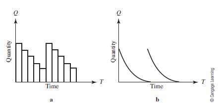
Discuss the assumptions implicit in the two graphical models depicted in Figure 13.8. Suggest scenarios in which each model might apply. How would you determine theFigure 13.8submodel for demand in
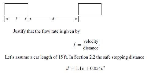
What are the optimal speed and safe following distance that allow the maximum flow rate (cars per unit time)? The solution to the problem would be useful in controlling trafc in tunnels, for roads
``An Application of Calculus in Economics: Oligopolistic Competition,'' by Donald R. Sherbert, UMAP 518. The author analyzes a number of mathematical models that investigate the competitive structure
Using the basic nonlinear model, y = axb t the following data set and provide the model, a plot of the data and the model, and a residual plot: 100 125 125 150 150 200 200 250 250 300 300 350 400
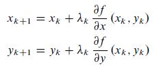
Write a computer code to perform the gradient method of steepest ascent algorithmusing the Golden Section Search Method (presented in Section 7.6) to maximize thefunction:to obtain λ=λk at each
Research the requirements for the necessary and sufficient conditions for the method of Lagrange multipliers and prepare a 10-minute talk.
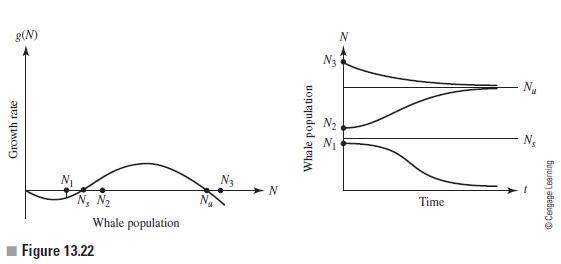
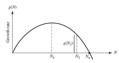
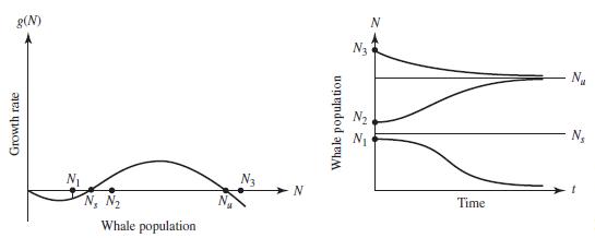
Argue that for many species, a minimum population level is required for survival. Give several examples. Call this minimum survival level Ns. Suggest a simple cubic growth submodel meeting these
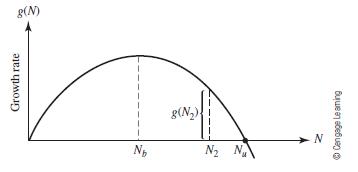
One of the key assumptions underlying the models developed in this section is that the harvest rate equals the growth rate for a sustainable yield. The reproduction submodelsin Figures 13.19 and
One of the difficulties in managing a fishery in a free enterprise system is that excess capacity may be created through over capitalization. This happened in 1970 when the capacity of the Peruvian
Taxation is appealing from a theoretical perspective because with a properly designed tax, desired goals can be achieved through normal market forces rather than by some artificial method (such as
In humans, the hydrostatic pressure of blood contributes to the total blood pressure. The hydrostatic pressure P is a product of blood density, height h of the blood column between the heart and some
Complete the requirements of ``Keeping Dimension Straight,'' by George E. Strecker, UMAP 564. This module is a very basic introduction to the distinction between dimensions and units. It also
Using dimensional analysis, find a proportionality relationship for the centrifugal force F of a particle in terms of its mass m, velocity v, and radius r of the curvature of its path.
In fluid mechanics, the Reynolds number is a dimensionless number involving the fluid velocity v, density ρ , viscosity μ, and a characteristic length r. Use dimensional analysis to find the
The lift force F on a missile depends on its length r, velocity v, diameter δ , and initial angle θ with the horizon; it also depends on the densityρ , viscosity μ, gravity g, and speed of sound
The height h that a fluid will rise in a capillary tube decreases as the diameter D of the tube increases. Use dimensional analysis to determine how h varies with D and the specific weight w and
Use a model employing a differential equation to predict the period of a simple frictionless pendulum for small initial angles of displacement. (Let sin θ= θ.) Under these conditions, what should
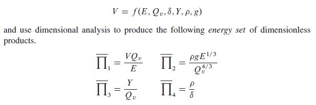
For the explosion process and material characteristics discussed in Problem 3, consider:Data from problem 3Consider a zero-depth burst, spherical explosive in a soil medium. Assume the value of the
Consider predicting the pressure drop Δp between two points along a smooth horizontalpipe under the condition of steady laminar flow. Assume:where s is the control distance between two points in the
It is desired to study the velocity v of a fluid flowing in a smooth open channel. Assume that:where r is the characteristic length of the channel cross-sectional area divided by the wetted
Use the polar coordinate substitution x = r cos θ and y = r sin θ in Equation (15.6) to show that a doubling of y0 causes a doubling of r for every fixed θ. Show that if y0 increases, then y =
For Problems 2 and 3, find the natural cubic splines that pass through the given data points. Use the splines to answer the requirements. X y 0 + 0.00 /6 /3 0.50 0.87 /2 1.00 2/3 0.87 5/6 0.50 T 0.00
y ∝ ex y X 6 15 42 114 311 845 2300 6250 17000 46255 1 2 3 4 5 6 7 8 9 10
y ∝ x3 y 0 1 2 6 14 24 37 58 82 114 1 2 3 4 5 6 7 8 9 10
y ∝ x2 y X 4 11 22 35 56 80 107 140 175 215 1 2 3 4 5 6 7 8 9 10
d ∝ v2 d V 22 28 33 39 44 50 55 61 66 72 77 20 25 30 35 40 45 50 55 60 65 70
y ∝ x3 y X 19 25 32 51 57 71 113 141 123 187 192 205 252 259 294 17 19 20 22 23 25 28 31 32 33 36 37 38 39 41
Force ∝ Stretch Force Stretch 10 20 30 40 50 60 70 80 90 19 57 94 134 173 216 256 297 343
Consider Example 1, A Car Rental Company. Experiment with different values for the coefficients. Iterate the resulting dynamical system for the given initial values. Then experiment with different
``Epidemics,'' by Brindell Horelick and Sinan Koont, UMAP 73. This unit poses two problems: (1) At what rate must infected persons be removed from a population to keep an epidemic under
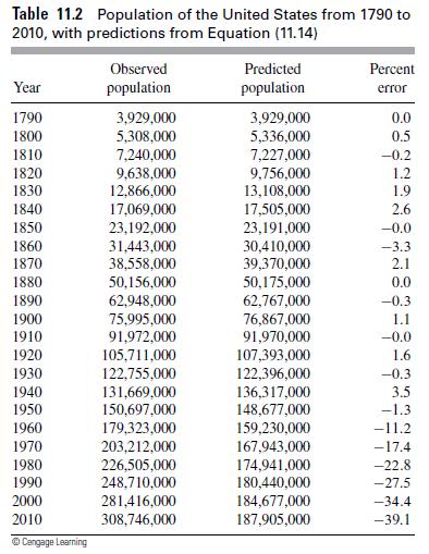
Using the data for the U.S. population in Table 11.2, estimate M, r, and t∗ using the same technique as in the text. Assume you are making the prediction in 1951 using a previous census. Use the
From the Further Reading, on Nash arbitration. The mathematics of Nash arbitration is to find Point N inside the convex payoff polygon that maximizes (x– x∗) (y– y∗) subject to
Pick a scenario of interest that fits into a game theory model. Decide the players, the strategies, and the values for the payoff matrix and then use the techniques in this chapter to find the
Assume we have two countries at war, Red and Blue. Assume Red wants to destroy Blue's base, and Red has four missiles, two with real warheads and two with dummy warheads. Blue defends its base and
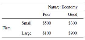
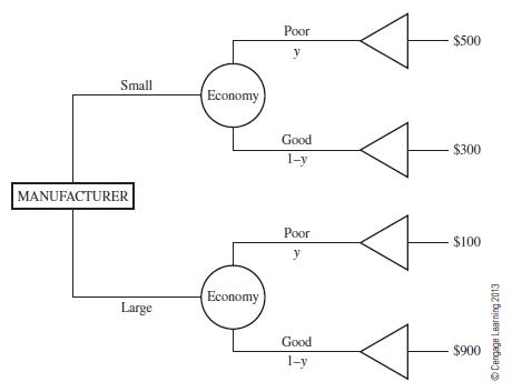
Refer to Example 1; formulate and then solve both the firm's game and the economy's game algebraically.Data from example 1Let's consider the following scenario. A manufacturing firm is considering
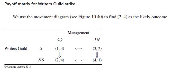
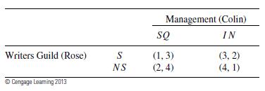
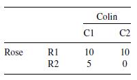
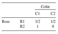
Using the definition provided for the movement diagram, determine whether the following zero-sum games have a pure strategy Nash equilibrium. If the game does have a pure strategy Nash equilibrium,
Consider a firm handling concessions for a sporting event. The firm's manager needs to know whether to stock up with coffee or cola and is formulating policies for specific weather predictions. A
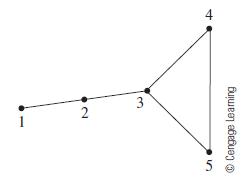
Consider the graph shown in Figure 8.36.Figure 8.36a. Find a minimum vertex cover in the graph in Figure 8.36. 5 2 3 Cengage Learning
A basketball coach needs to find a starting lineup for her team. There are five positions that must be filled point guard: (1) Shooting guard.(2) Swing. (3) Power forward. (4) And center. (5)
Solve the softball manager's problem (both versions) from the Introduction to this chapter.
Perform a complete sensitivity analysis (objective function coefficients and right-hand-side values) of the wooden toy soldier problem in Section 7.2 (Problem 1).Data from problem 7.2Consider a
Write a computer code to perform the basic simplex algorithm. Solve Problem 3 using your code.
Examine closely the system of equations that result when you fit the quadratic in Problem 3. Suppose c2 = 0. What would be the corresponding system of equations? Repeat for the cases c1= 0 and c3 =
For the data collected in the tape recorder problem (Sections 4.2 and 4.3) relating the elapsed time with the counter reading, construct the natural spline that passes through the data points.
Construct a computer code for determining the coefficients of the natural splines that pass through a given set of data points. See Burden and Faires, cited earlier in this chapter, for an efficient
Select a project from Projects 1–7 in Section 2.3 and use least squares to fit your proposed proportionality model. Compare your least-squares results with the model used from Section 2.3. Find the
Describe in detail the data you would like to obtain to test the various submodels supporting Model (2.21). How would you go about collecting the data?Data from model (2.21)where k5 = k2+k4. Note
Consider the models W ∝ l2g and W ∝ g3. Interpret each of these models geometrically. Explain how these two models differ from Models (2.11) and (2.13), respectively. In what circumstances, if
Design a plastic disk to perform the calculations given by Model (2.13).Data from model 2.13 This computation leads to the model W = 0.0196/g (2.13)
An object is sliding down a ramp inclined at an angle of θ radians and attains a terminal velocity before reaching the bottom. Assume that the drag force caused by the air is proportional to Sv2,
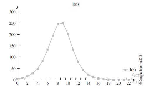
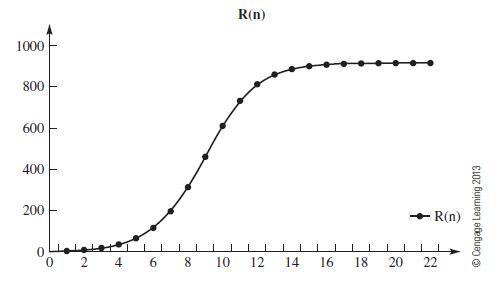
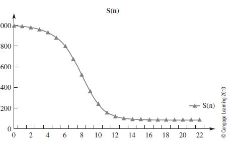
Find the equilibrium values for model (1.11).Data from equilibrium values for model (1.11) R(n + 1) = R(n) + 0.61 (n) I(n+1) = 1 (n)- 0.61 (n) +0.0014071 (n)S(n) S(n + 1) = S(n) - 0.001407S(n)I (n)
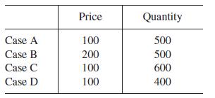
An economist is interested in the variation of the price of a single product. It is observed that a high price for the product in the market attracts more suppliers. However, increasing the quantity
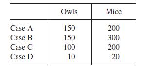
Suppose the spotted owls' primary food source is a single prey: mice. An ecologist wishes to predict the population levels of spotted owls and mice in a wildlife sanctuary. Letting Mn represent the
Again, consider Problem 12 above. Now assume that each month you charge $105. Determine what monthly payment p will pay off the card in:a. Two years.b. Four years.Data from problem 12Your current
For Problems 7–10, formulate a dynamical system that models change exactly for the described situation.Your grandparents have an annuity. The value of the annuity increases each month by an
By substituting n = 0; 1; 2; 3, write out the first four algebraic equations represented by the following dynamical systems:a. b. an+1 = 3an, ao = 1
By examining the following sequences, write a difference equation to represent the change during the nth interval as a function of the previous term in the sequence.a. b. {2, 4, 6, 8, 10, ...}
Write out the first five terms a0–a4 of the following sequences:a. An+1 = 3an, a0 = 1.b. An+1 = 2an + 6, a0 = 0.
When interest is compounded, the interest earned is added to the principal amount so that it may also earn interest. For a 1-year period, the principal amount Q is given by:where i is the annual
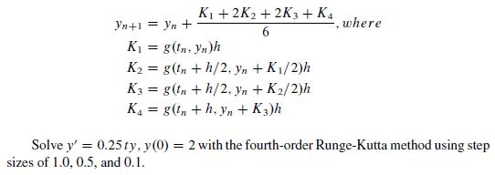
When we use the average of the estimates of the derivatives at the end points, we can improve the approximation to the solution. A class of approximation techniques that estimates derivatives at
y cos2 x dy + sin x dx = 0In Problems 1–8, solve the separable differential equation using u-substitution.
y′ = (y/x)2In Problems 1–8, solve the separable differential equation using u-substitution.
y′ = xyex2In Problems 1–8, solve the separable differential equation using u-substitution.
(x2 + x–2) dy + 3y dx = 0In Problems 17–24, solve the separable differential equation using partial fractions.
9y dx– (x–1)2(x + 2) dy = 0In Problems 17–24, solve the separable differential equation using partial fractions.
ex dy + (y3 –y2) dx = 0In Problems 17–24, solve the separable differential equation using partial fractions.
√1–y2 dx + (x2 –2x + 2) dy = 0In Problems 17–24, solve the separable differential equation using partial fractions.
(2x– x2) dy + e–y dx = 0In Problems 17–24, solve the separable differential equation using partial fractions.
√2xy dy/dx = 1In Problems 25–32, solve the separable differential equation.
(ln x) dx/dy = xyIn Problems 25–32, solve the separable differential equation.
x2 dy + y(x–1) dx = 0In Problems 25–32, solve the separable differential equation.
yex dy – (e–y + e2x–y) dx = 0In Problems 25–32, solve the separable differential equation.
(x ln y) y′ = (x + 1/y)2In Problems 25–32, solve the separable differential equation.
y′= sin–1 x/2y ln yIn Problems 25–32, solve the separable differential equation.
y′ D e-y – xe-y cos x2In Problems 25-32, solve the separable differential equation.
(1 + x + xy2 + y2) dy = (1–x)–1 dxIn Problems 25-32, solve the separable differential equation.
y–2 dx/dy = ex/e2x + 1, y (0) = 1In Problems 33-39, solve the initial value problem.
dy/dx+ xy = x, y (1) = 2In Problems 33-39, solve the initial value problem.
y′ –2y = 1, y (2) = 0In Problems 33-39, solve the initial value problem.
2(y2 –1) dx + sec x csc x dy = 0, y (π /4) = 0In Problems 33-39, solve the initial value problem.
dP/dt + P = P tet , P (0) = 1In Problems 33-39, solve the initial value problem.
dP/dt = (P2 – P) t–1, P (1) D= 2In Problems 33-39, solve the initial value problem.
x dy – (y+√y) dx = 0, y (1) = 1In Problems 33-39, solve the initial value problem.
Showing 1 - 100
of 698
1
2
3
4
5
6
7